A simple and interpretable performance measure for a binary classifier

Kindly reposted to KDnuggets by Gregory Piatetsky-Shapiro 

Preamble

The core application of machine learning models is a binary classification task. This appears in polyhedra of areas from medicine for diagnostic tests to credit risk decision making for consumers.  Techniques in building classifiers vary from simple decision trees to logistic regression and lately super cool deep learning models that leverage multilayered neural networks. However, they are mathematically different in construction and training methodology, when it comes to their performance measure, things get tricky. In this post, we propose a simple and interpretable performance measure for a binary classifier in practice. Some background in classification is assumed. 

Why ROC-AUC is not intepretable? 

PCC in Python (Author). 

De-facto standard in reporting classifier performance is to use Receiver Operating Characteristic (ROC) - Area Under Curve (AUC) measure. It originates from the 1940s during the development of Radar by the US Navy, in measuring the performance of detection.  There are at least 5 different definitions of what does ROC-AUC means and even if you have a PhD in Machine Learning, people have an excessively difficult time to explain what does AUC means as a performance measure. As AUC functionality is available in almost all libraries and it becomes almost like a religious ritual to report in Machine Learning papers as a classification performance. However, its interpretation is not easy, apart from its absurd comparison issues, see hmeasure.  

AUC measures the area under the True Positive Rate (TPR) curve as a function of the False Positive Rate (FPR) that are extracted from confusion matrices with different thresholds, $f(x)=y$ and  $\int_{0}^{1} f(x) dx = AUC$ whereby, y is TPR and x is FPR. Apart from a multitude of interpretations and easy to have confusions, there is no clear purpose of taking the integral over FPR. Obviously, we would like to have perfect classification by having FPR zero, but the area is not mathematically clear. Meaning that what is it as a mathematical object is not clear.

Probability of correct classification (PCC)

A simple and interpretable performance measure for a binary classifier would be great for both highly technical data scientist and non-technical stakeholders. The basic tenant in this direction is that the purpose of a classifier technology is the ability to differentiate two classes. This boils down to a probability value, Probability of correct classification (PCC). An obvious choice is so-called balanced accuracy (BA). This is usually recommended for unbalanced problems, even by SAS; though they used multiplication of probabilities. Here we will call BA as PCC and use addition instead, due to statistical dependence:
$PCC = \alpha TPR+ (1.0-\alpha TNR$

$TPR=TP/(ConditionPositive)=TP/(TP+FN)$
$TNR=TN/(ConditionNegative)=TN/(TN+FP)$
PCC tells us how good the classifier in detecting either of the class and it is a probability value, $[0,1]$. Note that, using total accuracy over both positive and negative cases are misleading, even if our training data is balanced in production, batches we measure the performance may not be balanced so accuracy alone is not a good measure. 

Attentive readers might note that this is about predictive values, Positive and Negative Predictive values, PPV and NPV match with the TPR and TNR respectively.

Production issues
Immediate question would be, how to choose the threshold in generating confusion matrix? One option would be to chose a threshold that maximizes PCC for production on the test set. To improve the estimation of PCC, resampling on the test set can be performed to get a good uncertainty.

Conclusion

We try to circumvent in reporting AUCs by introducing PCC, or balanced accuracy as a simple and interpretable performance measure for a binary classifier. This is easy to explain to a non-technical audience. An improved PCC, that takes into account better estimation properties can be introduced, but the main interpretation remains the same as probability of correct classification.  

Explore the notebook : pcc.ipynb

Please cite as follows:

 @misc{suezen20pcc, 

     title = {A simple and interpretable performance measure for a binary classifier}, 

     howpublished = {\url{https://memosisland.blogspot.com/2020/02/a-simple-and-interpretable-performance.html}, 

     author = {Mehmet Süzen},

     year = {2020}

}  

Bringing back Occam's razor to modern connectionist machine learning: A simple complexity measure based on statistical physics Cascading Periodic Spectral Ergodicity (cPSE)

Kindly reposted to KDnuggets by Gregory Piatetsky-Shapiro with the title Applying Occam's razor to Deep Learning 

Kindly reviewed by Cornelius Weber

Preamble: Changing concepts in machine learning due to deep learning

Occam's razor or principle of parsimony has been the guiding principle in statistical model selection. In comparing two models, which they provide similar predictions or description of reality, we would vouch for the one which is less complex. This boils down to the problem of how to measure the complexity of a statistical model and model selection. What constitutes a model, as discussed by McCullagh (2002) in statistical models context is a different discussion, but here we assume a machine learning algorithms are considered as a statistical model.  Classically, the complexity of statistical models usually measured with Akaike information criterion (AIC) or similar. Using a complexity measure, one would choose a less complex model to use in practice, other things fixed.

Figure 1: Arbitrary architecture, each node represents
a layer for a given deep neural network, such as
convolutions or set of units.  Süzen-Cerdà-Weber (2019)

The surge in interest in using complex neural network architectures, i.e., deep learning due to their unprecedented success in certain tasks,  pushes the boundaries of "standard" statistical concepts such as overfitting/overtraining and regularisation. 

Now Overfitting/overtraining is often used as an umbrella term to describe any unwanted performance drop off a machine learning model Roelofs et. al. (2019) and nearly anything that improves generalization is called regularization, Martin and Mahoney (2019).

A complexity measure for connectionist machine learning

Deep learning practitioners rely on choosing the best performing model and do not practice Occam's razor.  The advent of Neural Architecture Search and new complexity measures  

that take the structure of the network into account gives rise the possibility of practising Occam's razor in deep learning. Here, we would cover one of the very practical and simple measures called cPSE, i.e., cascading periodic spectral ergodicity. This measure takes into account the depth of the neural network and computes fluctuations of the weight structure over the entire network,  Süzen-Cerdà-Weber (2019) Figure 1. It is shown that the measure is correlated with the generalisation performance almost perfectly, see Figure 2.

Practical usage of cPSE

Figure 2: Evolution of PSE, periodic spectral ergodicity,
it is shown that complexity measure cPSE saturates
after a certain depth,  Süzen-Cerdà-Weber (2019)

The cPSE measure is implemented in Bristol python package, starting from version 0.2.6. If a trained network wrapped into a PyTorch model object, cPSE can be used to compare two different architectures. If two architectures give similar test performance, we would select the one with higher cPSE value. Lower the cPSE, more complex the model.

An example of usage requires a couple of lines, example measurements for VGG and ResNet are given in Süzen-Cerdà-Weber (2019):

from bristol import cPSE
import torchvision.models as models
netname = 'vgg11'
pmodel = getattr(models, netname)(pretrained=True)
(d_layers, cpse) = cPSE.cpse_measure(pmodel)

Conclusion and take-home message

Using a less complex deep neural network that would give similar performance is not practised by the deep learning community due to the complexity of training and designing new architectures. However, quantifying the complexity of similarly performing neural network architecture would bring the advantage of using less computing power to train and deploy such less complex models into production. Bringing back the Occam's razor to modern connectionist machine learning is not only a theoretical and philosophical satisfaction but the practical advantages for environment and computing time is immense.

Postscript : Appendix : Vanilla computation of cPSE

Recipe is quite easy to implement in practice: Get all weight matrices of your trained architecture as list of 2D matrices, special layers and biases subject to mapping, then:

from bristol import cPSE

spectrum_set = cPSE.get_eigenvals_layer_matrix_set(layer_matrices)

periodic_spectrum_set = cPSE.eigenvals_set_to_periodic(spectrum_set)

spectral_ergodicity_over_layers = cPSE.d_layers_pse(periodic_spectrum_set)

One should stop adding more layers where spectral_ergodicity_over_layers saturates to a constant value, i.e., decreasing curve.

A simple pedagogical one-line python code for the Fibonacci sequence with recursion (and memoization)

Fibonacci, Leonardo da Pisa
(Wikipedia)

Updated with memoization on 26 Feb 2020

Preamble

The Fibonacci sequence $F_{n} = F_{n-1} + F_{n-2}$ is famous for both artistic and pure mathematical curiosity as an integer sequence. A simple implementation of this sequence appears as a standard programmer's entry-level job question, along with finding factorial and greatest common divisor. In this short post, we will show how to implement $F_{n}$ with recursion in Python one-liner.

Fibonacci Recursion in Python

Here is a one-liner

f = lambda n : n if n < 2 else f(n-1)+f(n-2) ; [f(n) for n in range(0,13)]

Let's dissect the one line. $f$ is our function that computes the $nth$ member of the sequence in a recursive fashion.

For example, a recursion of $f$ at $n=3$ follows the following depth as recursive calls:

1. Upper level, n=3 : f(2)+f(1)
2. n=2 : f(1) + f(0) 
1. Returns 1+0 = 1
3. n=1 : f(1) 
1.  Returns 1
4. Returns 2

Recall that every recursion needs a termination condition, which is less than two in our case. The second part of one-liner after semi-column, which indicates another line,  is a simple list-comprehension to repeat the call to $f$ from 0 to 12. Resulting

 [0, 1, 1, 2, 3, 5, 8, 13, 21, 34, 55, 89, 144] 

Computational efficiency

To compute the sequence for a very large set, this implementation is obviously very slow. One would need to introduce caching within the recursion to avoid repeated computation.

Reading list for novice coders

• List comprehension originating from set builder notation.
• Lambda expressions so-called anonymous functions.
• Recursion, it is a beautiful concept in computer science.
• Range function in Python.

Conclusion

One of the most interesting programming tasks usually comes in implementing integer sequences. Note that Fibonacci day is celebrated on 23rd of November, the day this post is published.

Postscript: Time complexity, memoization version with timings

The complexity of 1 liner code above is $O(2^N)$, with caching it can be $O(N)$. Thanks to Tim Scarfe for pointing out Big-O complexities. The solution is to introduce caching, this is so-called memoization.

The following gives timing for $m=35$ without and with memoization. It is seen that memoization is almost  5 orders of magnitude faster and will actually memory efficient as well. For larger $m$ memoization version may return a value but without memoization, we would quickly overflow on recursive calls.

import time
m = 35

# no memoization
t0 = time.process_time()
f = lambda n : n if n < 2 else f(n-1)+f(n-2) ;  sfib = [f(i) for i in range(1,m)]
time.process_time() - t0

# memoization
t0 = time.process_time()
mem={1:1,2:2} ; f = lambda n : n if n < 2 else mem.get(n) if mem.get(n) else mem.update({n:f(n-1)+f(n-2)}) ; sfib_mem = [f(i) for i in range(1,m)]; sfib_mem = [1]+list(mem.values())
time.process_time() - t0
 

On modern data scientist: A blind empiricist is not a data scientist

As mentioned by Professor Pearl graciously on twitter 

Preamble

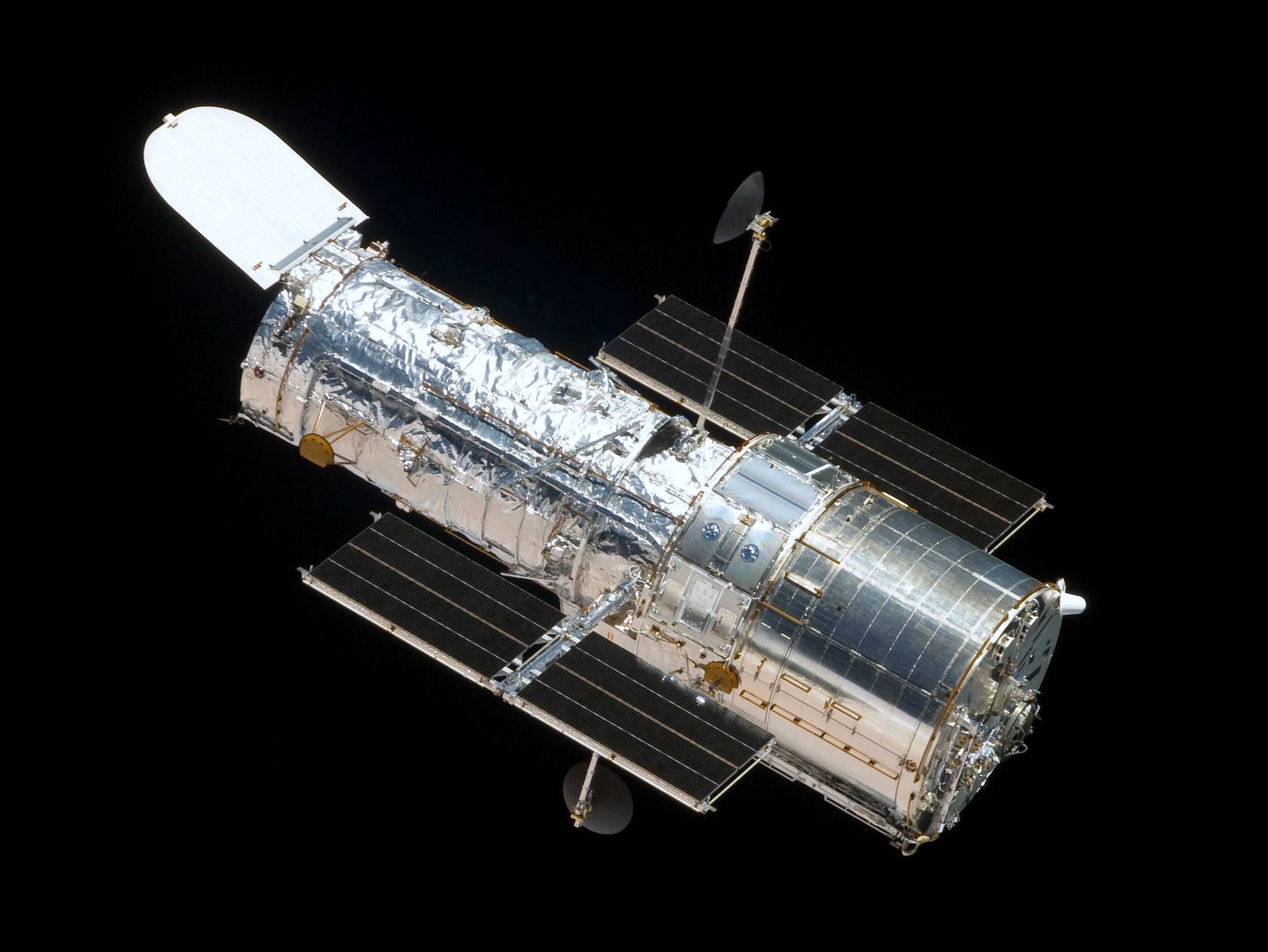
Hubble Space Telescope (Wikipedia)
Computational science is to
modern data scientist, as telescopes are
for astrophysics.

A better software developer than a statistician and better statistician than a software developer would have been a good definition for the early 2010s in identifying who would be a data scientist. In the late 2010s, trends changed dramatically, a data scientist is now identified as who can turn any set of data to run through machine learning libraries and getting a model to deploy for service.  Unfortunately, this blind empiricism is now considered as a data science practice in many industrial places and the term "scientist" lost its intellectual practice and turn into the mass hysteria of producing "junk science" blindly in the name of "democratisation of data science".

Who is the modern data scientist? 

Modern data science actually goes beyond statistics and machine learning. Modern data scientist practice computational science from dynamical systems to game theory or graph theory. One could think of such practice as applied mathematics or statistical physics as well.  For example, most of the neural networks is actually originating from statistical physics. In that sense, a modern data scientist is a computational scientist building mechanics of data.

1. The exploratory analysis goes beyond basic PCA or clustering to be able to form causal relationships or establish mechanics of the data.
2. Can express the mechanics of data in mathematical models and build parametric inference. Not all parameter estimations are learning.
3. Use machine learning algorithms from libraries by knowing the underlying algorithm and can relate this to the mechanics of data.
4. Build algorithms fusing above work.
5. Explainable and transparent work.
6. Document the findings as in the scientific paper and scientific software. 

Ignoring the above practice and treating data science similar to a web-based software development activity is not a fair practice and an immense waste of time. Organisations should understand that investing in data science means investing in the new computational science of building mechanics of data. Pushing the outcome of such a scientific practice to make a real-world impact lies in the novelty of scientist and as in any scientific funding, this is a very risky investment.

Misconception in democratisation of data science

The democratisation of data science does not mean that anyone should build learning or statistical models using machine learning libraries and put lots of data to get a black-box model as a blind empiricist. Democratisation was about the availability of tools and services at very low cost and open culture of transparency in algorithmic and software work.

Artificial Intelligence is modern data science

The separation of AI from the above definition of data science is not really clear. While AI combines the same characteristics to build so-called intelligent agents.

Conclusion

Having a perspective and understanding of what is modern data science about will help organisations better orient in building modern data science capabilities.

Postscript: Further reading and on the mechanics of data

We used a term the mechanics of data, it implies the effort to put in finding signatures of causal relationships and make sense of the correlations within the data. The reason is one of the core scientific methods that give rise to modern science lies in Newton-Leibniz mechanics. Coveney and his co-worker's deep dives in intricacies of practising science and data science.

• Big data: the end of the scientific method?
  Sauro Succi and Peter V. Coveney
  [article]
• Big data need big theory too
  Peter V. Coveney, Edward R. Dougherty and Roger R. Highfield
  [article]

Post-Postscript

Judea Pearl, a pioneering scientist on causal inference field, a quiet revolution in statistics and data science, Turing award laureate has similar critique on excessive empiricism. His post explains: 

Radical Empiricism and Machine Learning Research, which is also published as an article here: doi