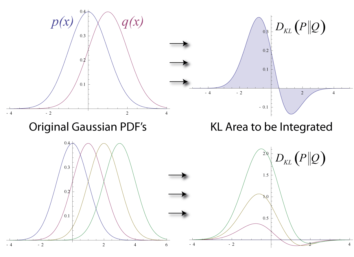
In this short tutorial, I show how to compute KL divergence and mutual information for two categorical variables, interpreted as discrete random variables.
${\bf Definition}$: Kullback-Leibler (KL) Distance on Discrete Distributions
 | |
|
$D_{KL} = D_{KL}\big({\it P}(A) || {\it Q}(B)\big)=\sum_{j=1}^{n} {\it P}(A=a_{j}) \log \Big( \cfrac{{\it P}(A=a_{j})}{{\it Q}(B=b_{j})} \Big)$
$\log$ is in base $e$.
${\bf Definition}$: Mutual Information on Discrete Random Variates
Two discrete random variables $X$ and $Y$, having realisations $X=x_{k}$ and $Y=y_{l}$, over $m$ and $n$ singletons $k=1,...,n$ and $l=1,...,m$ respectively, are given. Mutual information, $I(X;Y)$ is defined as follows,
$I(X;Y) = \sum_{k=1}^{n} \sum_{l=1}^{m} {\it R}(X=x_{k}, Y=y_{l}) \log \Big(\cfrac{ {\it R}(X=x_{k}, Y=y_{l}) }{ {\it R}(X=x_{k}) {\it R}(Y=y_{l})} \Big)$
$\log$ is in base $e$ and $R$ denotes probabilities.
${\bf Definition}$: Mutual Information on Discrete Random Variates with KL distance
Two discrete random variables $X$ and $Y$. Mutual information, $I(X;Y)$ is defined as follows,
$I(X;Y) = D_{KL} \Big( {\it R}(X, Y) || {\it R}(X) {\it R}(Y) \Big)$
${\bf Problem: Example}$: Given two discrete random variables $X$ and $Y$ defined on the following sample spaces $(a,b,c)$ and $(d,e)$ respectively. Write down the expression for the mutual information, I(X;Y), expanding summation.
${\bf Solution: Example}$:
$I(X;Y) = {\it R}(X=a, Y=d) \log \Big(\cfrac{ {\it R}(X=a, Y=d) }{ {\it R}(X=a) {\it R}(Y=d)} \Big) +$
${\it R}(X=b, Y=d) \log \Big(\cfrac{ {\it R}(X=b, Y=d) }{ {\it R}(X=b) {\it R}(Y=d)} \Big)+$
${\it R}(X=c, Y=d) \log \Big(\cfrac{ {\it R}(X=c, Y=d) }{ {\it R}(X=c) {\it R}(Y=d)} \Big)+$
${\it R}(X=a, Y=e) \log \Big(\cfrac{ {\it R}(X=a, Y=e) }{ {\it R}(X=a) {\it R}(Y=e)} \Big)+$
${\it R}(X=b, Y=e) \log \Big(\cfrac{ {\it R}(X=b, Y=e) }{ {\it R}(X=b) {\it R}(Y=e)} \Big)+$
${\it R}(X=c, Y=e) \log \Big(\cfrac{ {\it R}(X=c, Y=e) }{ {\it R}(X=c) {\it R}(Y=e)} \Big)$
${\bf Definition}$: Two discrete random variables $X$ and $Y$, having realisations $X=x_{k}$ and $Y=y_{l}$, over $m$ and $n$ singletons $k=1,...,n$ and $l=1,...,m$ respectively, are given. Two-way contingency table of realisations of $X$ and $Y$ along the same measured data points, $N$ observations, can be constructed by counting co-occurances, or cross-classifying factors. Normalizing the resulting frequency table will produce joint and marginal probabilities.
Y=y_{1} ... Y=y_{l} R(X)
X=x_{1} R(X=x_{1}, Y=y_{1}) ... R(X=x_{1}, Y=y_{l}) R(X=x_{1})
X=x_{2} R(X=x_{2}, Y=y_{1}) ... R(X=x_{2}, Y=y_{l}) R(X=x_{2})
... ... ... ... ...
X=x_{k} R(X=x_{k}, Y=y_{1}) ... R(X=x_{k}, Y=y_{1} R(X=x_{k})
R(Y) R(Y=y{1}) ... R(Y=y_{l})
Simulated example with R
1 2 3 4 5 6 7 8 9 10 11 12 13 14 15 16 17 18 | set.seed(3951824) # Table of counts (contingency) X <- sample(letters[1:3], 100, 1) Y <- sample(letters[4:5], 100, 1) t <- table(X,Y) tp <- t/100 # proportions tn <- tp/sum(tp) # normalized, joints p_x <- rowSums(tn) # marginals p_y <- colSums(tn) P <- tn Q <- p_x %o% p_y # P(X, Y) : bin frequency: P_i # P(X) P(Y) : bin frequency, Q_i mi <- sum(P*log(P/Q)) library(entropy) mi.empirical(t) == mi |
References
(KullbackLeibler57) Kullback, S.; Leibler, R.A. (1951). "On information and sufficiency". Annals of Mathematical Statistics 22 (1): 79–86.

8 comments:
Hu there.
I found this post very goood.
Is there some issue or typo with the R code command %o% that I do not know?
Thank you,
Nuno Edgar Fernandes
Hi Nuno,
Thanks.
%o% is an outer product. It is from R base, have a look at ?outer or from the manual outer.
Hi:
Nice example but as of january 2018 can't load entropy library, only EntropyEstimation, would that do it? Or how can i load it? Thanks in advance.
@Daniel What error message you had? entropy package is still available. You need to install it with install.packages("entropy"). Try a different CRAN mirror if you have issues. Sometimes mirrors can have issues in updating properly. If you want to use EntropyEstimation, use one of the KL or MI functions. Note that it uses a different estimator.
Hi
very useful post,this example is solved for two random variables. How it could be done if there are more than two random continuous variables. I am doing variable selection using mutual information based on entropy. please help and give some suggestions.
Thanks and regards
@Unkonwn For continuous case you need to take multi-dimensional integrals.
Thankyou msuzen
Thank you msuzen
Post a Comment