Why should there be no simultaneity rule for causal models?

Dominos in motion
(Wikipedia)

Preamble 

The definition of weighted directed graphs (wDAGs) provides a great opportunity to express causal relationships among given variates. Usually this is expressed as SCMs, Structural Causal Model or in more generally causal model. A given causal model can be expressed as set of simultaneous equations, given a direction for the equality, right to left , meaning $A=B$ implies B causes A to happen  $B \to A$ . Then what happens if A is a function of B and C, $A=f(B,C)$, then we say $ B \to A$ and $C \to A$ occurs simultaneously.  In this post we discuss this situation that there should be no simultaneity rule in causal models, regardless of if they are not time-series models.

Understanding  causal models

Basic definition of a causal model follows a functional form with set of equations, realistically with added noise. The models forms a weighted Directed Acyclic Graphs (wDAGs) visually. Here is the mathematical definition due to Pearl (Causality 2009), we made it a bit more coarser in this definition: 

Definition (Causal Model) : Given set of $n$-variables $X \in \mathbb{R}^{n}$, two subsets of $X= x_{1} \cup x_{2}$, they can form set of equations $x_{2}=f(x_{1}; \alpha; \epsilon)$,  $\alpha$ being the causal effect sizes on $x_{1}$ as causes of $x_{2}$ with some noise $\epsilon$. This corresponds to a $wDAG$ formed among $X$ with weights $\alpha$. So that there is a graph $\mathscr{G}(X, \alpha)$ representing this set of equations, where by equality put direction from right to the left side of the equation. 

However this definition does not set any constraints on the values of $\alpha$. Any two or more values of $\alpha$-s can be equivalent on the same path within $X$. This implies an interestingly that there would be set of variates simultaneously causes the same thing. It sounds plausible and physically possible to a degree within Planck-time. However, this brings an ambiguity of breaking ties in ordering events.

Perfect Causal Ordering

Given wDAG as a causal model induces causal ordering among all members of $X$. As we defined how this can be achieved in a recent post: Practical causal ordering. In this context, perfect causal ordering implies  $\alpha$ values within the first order paths to a given end variable are different. Mathematically speaking a definition follows. 

Definition (No simultaneity rule) Given all $k$ triplets ($x_{i}, y, \alpha_{i}$), that $x_{i}$ is one of the causes of $y$, and $\alpha_{i}$ causal effect sizes, all $\alpha_{i}$ are different numbers, inducing a perfect causal ordering.

This rule ensures we don't need to break ties randomly as causal ordering is established uniformly.

Conclusion: Importance of no simultaneity 

By this definition we ruled out any simultaneous causes. This may sound too restrictive for modelling but this impacts decision making significantly; ranking causes of an outcome will impact how to prioritise the policy in addressing the outcome, i.e., such as medical intervention to prevent first cause. Also, it may not be feasible to intervene simultaneous causes. Hence, establishing primary causes in order is paramount in decision making and execution of any reliable policy.

Further reading

• looper : Causality Resource 
• Looper Nuggets 1 (LN1) : Definition of wDAGs with no simultaneity rule.

Please cite this article as: 

 @misc{suezen23nos, 

     title = {Why should there be no simultaneity rule for causal models?}, 

     howpublished = {\url{https://memosisland.blogspot.com/2023/11/causal-model-simultaneous.html}, 

     author = {Mehmet Süzen},

     year = {2023}

}

  

Ising-Conway lattice-games: Understanding increasing entropy

Preamble

The entropy is probably one of the most difficult physical concepts to grasp. Its inception roots in efficiency of engines and foundational connection to multi-particle classical mechanics to thermodynamics,  i.e., kinetic theory to thermo-statistics. However, computing entropy for a physical systems is a difficult task, as most of the real-physical systems lacks the explicit formulation. Apart from advanced simulation techniques that invokes thermodynamical expressions, pedagogically accessible and physically plausible system is lacking in the literature. Addressing this, we explore here, recently proposed Ising-Conway Games.

Figure: Evolution of Ising-Conway
Game  (arXiv:2310.01458)

Ising-Conway Lattice-Games (ICG)

Ising-Lenz model is probably one of the landmark models in physics, remarkably provides beyond its idealised case of magnetic domains,  now impacts even quantum computational research. However, computing entropy of Ising-Lenz models are still quite difficult. On the other hand, Conway introduce a game with simple rules generating complexity in various orders, via simple dynamical rules. By analogy to these two modelling approach,  we recently introduce game like physical system of spins or lattice sides on a finite space with constraints. This gives a physically plausible dynamics but simpler dynamical evolution to generate the trajectories. Because vanilla Ising-Models requires more complicated Monte Carlo techniques.  Here is the configuration and dynamics of Ising-Conway games,

1. $M$ sites as a fixed space.
2. $N$ occupied sites, or 1s.  
3. Configuration $C(M,N,t)=C(i)$ over time changes. But at $t=0$ all occupied sites live in at the corner.
4. Configuration can only change to neighbouring sites if they are empty. This is closely related to spin-flip dynamics of the Ising Model. 
5. No sites occupy the same lattice cell, Pauli exclusion
6. Should be contained within $M$ Cell.

An example evolution is shown on the Figure.

Defining ensemble Entropy on ICG

Now we are in position to define the entropy for ICGs, which easy to grasp conceptually and computationally.  $C(i, t) \in \{1,0\}$ defines the states of  the game. We build an ensemble at a given time $t$ by defining a region enclosed by 1s.  Then dimensionality of the ensemble  $ k(t) = argmax[\mathbb{I}(C(i))] - argmin [\mathbb{I}(C(i)) ]$. Here,  $\mathbb{I}$ returns index of $1$s on the lattice. This ensemble closely track maximum entropy of the system at a given time. 

Conclusions

A new game-like system that helps us to understand entropy increase that has a plausible physical characteristics that one can easily simulate.

Further reading

• H-theorem do-conjecture, M.Süzen, arXiv:2310.01458
• Effective ergodicity in single-spin-flip dynamics, Mehmet Süzen. Phys. Rev. E 90, 03214 url
• do_ensemble module provides such simulation via simulate_single_spin_flip_game  from the repo h-do-conjecture 

Please cite as 

 @misc{suezen23iclg, 

     title = {Ising-Conway lattice-games: Understanding increasing entropy}, 

     howpublished = {\url{https://memosisland.blogspot.com/2023/10/ising-conway-games-entropy-increase.html}}, 

     author = {Mehmet Süzen},

     year = {2023}

}  

Practical causal ordering: Why weighted-Directed Acyclic Graphs (DAGs) are powerful for causal inference?

Preamble 

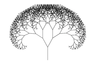
Fractal Tree (Wikipedia)

A quiet causal inference revolution is underway in industry. We see immense success of transformers deep learning architectures. However their success should also be attributed to causal modelling. Large Language Models (LLMs), specially closed-sourced ones, elevates their performance with encoding causal mechanism with human designed deep learning components, i.e., innovative layers such as causal convolutions with multi-head self-attention layers. Now a classical approach,  one of the corner-stone of causality, is expressing modelling variates' causal relationships with  Directed Acyclic Graphs (DAGs). This lead to causal analysis and preserving ordering. In this short tutorial, we cover these without graph theoretic language for practical causal ordering.

Understanding weighted Directed Acyclic Graphs (wDAGs) as causal data structure  

We first define what is a directions and weights. Providing a notational definition via tuples of objects.    

Definition (wDAG): A weighted Directed Acyclic Graph (wDAG)  $\mathscr{G_{c}}$  is defined as set of ordered triplets of weights and connected random variables, such that, $k$th  triplet $(w_{k}, x_{i}, x_{j})$ where by $w_{k} \in \mathbb{R}$ is the weight, an effect size, between two variates that $x_{i}$ effects $x_{j}$. There are constraints : 

(i) No cyclic effects can be defined, necessarily $x_{i}$ can not be equal to $ x_{j}$.

(ii) If there is a definition,  $(w_{k}, x_{i}, x_{j})$ the reverse can't be defined, i.e.,  so that $(w_{k}, x_{j}, x_{i})$ does not exist.    

(iii) No two causal effects sizes can't be exactly equal, $w_{k}$ can not be equal to $w_{l}$, from the same causal variable,  meaning no simultaneous events caused by the same random variable. This prevents ambiguity of ordering and random tie-breaks are unnatural.

This definition is practical and do not introduce any graph theory jargon. We left the sizes of indices as an exercise. 

Inducing Causal Order via wDAGs

By the very definition of wDAGs, the power of this definition is one can construct causal ordering. 

Definition (Causal Ordering from wDAG): Given $\mathscr{G_{c}}$, we can construct causal ordering among random variates $O(i)$ for $x_{i}$ using directionality and weights from  $\mathscr{G_{c}}$:

(i) if there exist a triplet  $(w_{k}, x_{i}, x_{j})$, then ordering $x_{j} \succ x_{i}$, implies $x_{j}$ occurred before $x_{j}$, or cause of $x_{i}$ was $x_{j}$

(ii) if there are two or more triplets having the same first variates, ordering is induces by the effect size $w_{k}$ among them.

To provide a simple example, let's say we formed  a wDAG, $\mathscr{G_{c}} = \{ (0.1, x_{1}, x_{2}),(0.2, x_{1}, x_{3}), (1.1, x_{2}, x_{4})  \}$ then the following causal ordering is established  $x_{1} \succ x_{3} \succ x_{2} \succ x_{4}$, note the ordering of $x_{3}$ that took precedence on $x_{2}$ due to its weight.

Why LLMs with causal ordering are so successful?

Probably not very well spelled property of LLMs are having causal layers with deep learning elevating their ability to capture causal ordering in natural language so well, not only sequence. This is still in infancy from research perspective as LLMs are biologically not plausible engineered software systems act as lossy knowledge compressors, lossy part usually identified as hallucination. 

Conclusion

We introduce basic definition of wDAGs without heavy graph theory jargon and provide hints on why causal ordering with wDAGs has an immense contribution in constructing useful LLMs.

Further reading

• looper : Causality Resource List. [link]
• Pearl et. al. Causal Inference in Statistics [link]
• Shimizu et. al., A Linear Non-Gaussian Acyclic Model for Causal Discovery [link]
• Hamad, et. al, Dilated causal convolution with multi-head self attention for sensor human activity recognition [link].
• Lui et. al DecBERT: Enhancing the Language Understanding of BERT with Causal Attention Masks [link]

Please cite as follows:

 @misc{suezen23pco, 

     title = {Practical causal ordering: Why weighted-Directed Acyclic Graphs (DAGs) are powerful for causal inference? }, 

     howpublished = {\url{https://memosisland.blogspot.com/2023/09/causal-ordering-dags-.html}}, 

     author = {Mehmet Süzen},

     year = {2023}

}  

Postscript Notes

Last Update 30 Oct 2024

• Transformers mathematically mimics wDAGs, i.e., induce causal ordering among distributed representations via “Attention” i.e., weighting inputs and linking them to different types of output sequences.  
• Directed Acyclic Graphs (DAGs), are actually build implicitly by transformer architectures. This lead to causal analysis and preserving ordering of most meaningful word embeddings in an empirical level, i.e., heuristic causality bound by data-driven model with inductive bias of the modeller (LLM trainer). Striking enough, it is possible to express these relationships using triplet notation without Graph Theory, and that’s what attention layer store rather than graph.
• The primary  driver in this is not that it can only place an attention to certain portions of the embedded vector space for approximating  the separation of meaning. These data processing instructions actually builds a causal mappings among sub-spaces, i.e., a causal ordering among embedding sub-spaces. In short, transformers are heuristically executing causal discovery.  
• Transformers in the context of machine translations performs 'causal graph discovery' heuristically, inducing causal ordering. That's why they exceeded previous translation architectures.
• Grateful to see Judea Pearl's kind note on this via twitter. "What's the input? Statistical data or human authored texts? What are the assumptions behind the discovery?" 
• This is critical as not to jump in conclusion that these neural network layers can do causal discovery automatically, but rather in human supervised conditions. The answer was, "Assumption is using an established causal model -human text/translation, directionality is already established. Then transformer compute weights on this graph. Other enabler is word embeddings & large examples. Can't do causal inference as in SCMs, still a statistical model."

•  Self-attention for LLMs acts as casual discovery machines over human experience

  The success of transformers deep learning architecture can also be attributed to causal modelling. But how?  Probably the most prominent  application of transformers in machine translation. As translation models trained on human translated data

  Causality is inbuilt in these datasets and transformers behave as causal discovery layers. We could imagine weights on the translation matrix and other query matrices as DAGs, as connection between connectivity matrices and graphs are well known. Directionality is dictated by asymmetric weights. This manifest as causal analysis  preserving ordering of most meaningful words embeddings empirically i.e., heuristic causality. This can be demonstrated by triplets without graph theoretic notation, that would induce as causal ordering discovery.

  Causal set theory is also quite striking in quantum gravity. DAGs appear as Partially-ordered sets of events in Planck-scale relativistic events within the discrete space-time. Monograph by Benjamin Dribus, Discrete Causal Theory, Springer (2017)

  
  

Full cross-validation and generating learning curves for time-series models

Kindly reposted to KDnuggets by Gregory Piatetsky-Shapiro

Preamble

Time-series analysis is needed almost in any quantitative field and real-life systems that collects data over time, i.e., temporal datasets. Building predictive models on temporal datasets for future evolution of systems in consideration are usually called forecasting. The validation of such models deviates from the standard holdout method of having random disjoint splits of train, test and validation sets used in supervised learning. This stems from the fact that time-series are ordered and order induces all sorts of statistical properties that should be retained. For this reason, applying direct cross-validation to time-series model building is not possible and only restricted to out-of-sample (OOS) validation, using the end-tail of a temporal set as a single test set. A recent work proposed an approach that overcomes the known limitation achieving full cross-validation for time-series. The approach opens up for a possibility to produce learning curves for the time-series models as well, which is usually also not possible due to similar reasons.

Reconstructive Cross-validation (rCV) : A meta-algorithm design principles

rCV is proposed recently in the paper titled Generalised learning of time-series: Ornstein-Uhlenbeck processes. The design principles of rCV for time-series aims at the following principles:

   Figure 1 : rCV meta-algorithm for time-series
cross-validation and learning curves.

1. Logically close to standard cross-validation: Arbitrary test-set size and number of folds. 
2. Preserve correlations and data order. 
3. Does not create absurdity of predicting past from the future data. 
4. Applicable in generic fashion regardless of learning algorithm. 
5. Applicable to multi-dimensional time-series. 
6. Evaluation metric agnostic.

Idea of introducing missing-data  : Temporal cross-validation and learning curves

The key idea of rCV is to create cross-validation sets via creating missing-data sets K-times, as in K-fold, with a given degree of missing ratio, i.e., random data point removal. Each fold will have disjoint set of missing data points. By an imputation method, we would fill out the K-disjoint missing data sets and generate K-different training datasets.  This would allow us to have K-different models and we could measure the generalised performance of the modelling approach by testing the primary models prediction on the Out-of-sample (OOS) test set. To avoid confusion about what is a model?, what we are trying to achieve is to find out hypothesis, i.e., the modelling approach.  By changing the ratio of missing data and repeating the cross-validation exercise will yield to set of ratio of missing-missing data introduced and their corresponding rCV errors, the plot is nothing but a learning-curve from supervised learning perspective.  Note that the imputation and prediction models are different models. The primary model we are trying to build is the prediction model we used for producing OOS predictions. The procedure is summarised in Figure 1. 

    Figure 2 : Synthetic data and reconstructions. 

Show-case with Gaussian process models on Ornstein-Uhlenbeck processes

To demonstrate the utility of rCV, the mentioned paper uses a synthetic data generated by Ornstein-Uhlenbeck process, i.e., Gaussian process with certain parameter setting.  Figure 2, shows the synthetic data and example locations of generated missing-data sets's reconstruction errors. Figure 3 shows learning curves depending on the different ratios of missing data setting. 

    Figure 3: Learning curves for the Gaussian Process model
generated by rCV.

Conclusion

rCV provides logically consistent way of practicing cross-validation in time-series. It is usually not possible to produce learning-curves on the same time-window for time-series model: by using rCV with different ratio missing data achieves this as well. rCV paves way to do generalised learning for time-series.

Further Reading

Apart from the paper Generalised learning of time-series: Ornstein-Uhlenbeck processes. the results can be reproduced with the Python prototype implementation,  here.