In this short tutorial, I show how to compute KL divergence and mutual information for two categorical variables, interpreted as discrete random variables.
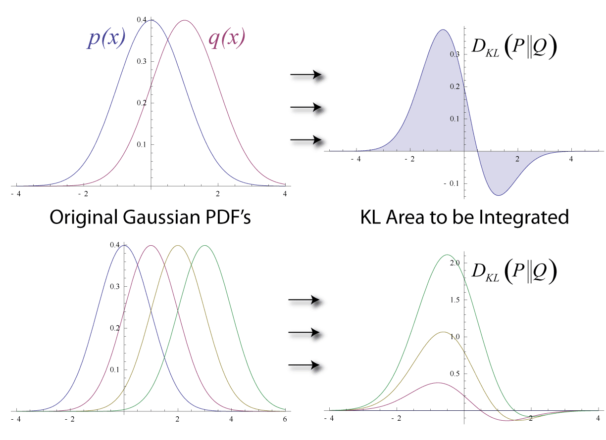
${\bf Definition}$: Kullback-Leibler (KL) Distance on Discrete Distributions
 | |
|
$D_{KL} = D_{KL}\big({\it P}(A) || {\it Q}(B)\big)=\sum_{j=1}^{n} {\it P}(A=a_{j}) \log \Big( \cfrac{{\it P}(A=a_{j})}{{\it Q}(B=b_{j})} \Big)$
$\log$ is in base $e$.
${\bf Definition}$: Mutual Information on Discrete Random Variates
Two discrete random variables $X$ and $Y$, having realisations $X=x_{k}$ and $Y=y_{l}$, over $m$ and $n$ singletons $k=1,...,n$ and $l=1,...,m$ respectively, are given. Mutual information, $I(X;Y)$ is defined as follows,
$I(X;Y) = \sum_{k=1}^{n} \sum_{l=1}^{m} {\it R}(X=x_{k}, Y=y_{l}) \log \Big(\cfrac{ {\it R}(X=x_{k}, Y=y_{l}) }{ {\it R}(X=x_{k}) {\it R}(Y=y_{l})} \Big)$
$\log$ is in base $e$ and $R$ denotes probabilities.
${\bf Definition}$: Mutual Information on Discrete Random Variates with KL distance
Two discrete random variables $X$ and $Y$. Mutual information, $I(X;Y)$ is defined as follows,
$I(X;Y) = D_{KL} \Big( {\it R}(X, Y) || {\it R}(X) {\it R}(Y) \Big)$
${\bf Problem: Example}$: Given two discrete random variables $X$ and $Y$ defined on the following sample spaces $(a,b,c)$ and $(d,e)$ respectively. Write down the expression for the mutual information, I(X;Y), expanding summation.
${\bf Solution: Example}$:
$I(X;Y) = {\it R}(X=a, Y=d) \log \Big(\cfrac{ {\it R}(X=a, Y=d) }{ {\it R}(X=a) {\it R}(Y=d)} \Big) +$
${\it R}(X=b, Y=d) \log \Big(\cfrac{ {\it R}(X=b, Y=d) }{ {\it R}(X=b) {\it R}(Y=d)} \Big)+$
${\it R}(X=c, Y=d) \log \Big(\cfrac{ {\it R}(X=c, Y=d) }{ {\it R}(X=c) {\it R}(Y=d)} \Big)+$
${\it R}(X=a, Y=e) \log \Big(\cfrac{ {\it R}(X=a, Y=e) }{ {\it R}(X=a) {\it R}(Y=e)} \Big)+$
${\it R}(X=b, Y=e) \log \Big(\cfrac{ {\it R}(X=b, Y=e) }{ {\it R}(X=b) {\it R}(Y=e)} \Big)+$
${\it R}(X=c, Y=e) \log \Big(\cfrac{ {\it R}(X=c, Y=e) }{ {\it R}(X=c) {\it R}(Y=e)} \Big)$
${\bf Definition}$: Two discrete random variables $X$ and $Y$, having realisations $X=x_{k}$ and $Y=y_{l}$, over $m$ and $n$ singletons $k=1,...,n$ and $l=1,...,m$ respectively, are given. Two-way contingency table of realisations of $X$ and $Y$ along the same measured data points, $N$ observations, can be constructed by counting co-occurances, or cross-classifying factors. Normalizing the resulting frequency table will produce joint and marginal probabilities.
Y=y_{1} ... Y=y_{l} R(X)
X=x_{1} R(X=x_{1}, Y=y_{1}) ... R(X=x_{1}, Y=y_{l}) R(X=x_{1})
X=x_{2} R(X=x_{2}, Y=y_{1}) ... R(X=x_{2}, Y=y_{l}) R(X=x_{2})
... ... ... ... ...
X=x_{k} R(X=x_{k}, Y=y_{1}) ... R(X=x_{k}, Y=y_{1} R(X=x_{k})
R(Y) R(Y=y{1}) ... R(Y=y_{l})
Simulated example with R
1 2 3 4 5 6 7 8 9 10 11 12 13 14 15 16 17 18 | set.seed(3951824) # Table of counts (contingency) X <- sample(letters[1:3], 100, 1) Y <- sample(letters[4:5], 100, 1) t <- table(X,Y) tp <- t/100 # proportions tn <- tp/sum(tp) # normalized, joints p_x <- rowSums(tn) # marginals p_y <- colSums(tn) P <- tn Q <- p_x %o% p_y # P(X, Y) : bin frequency: P_i # P(X) P(Y) : bin frequency, Q_i mi <- sum(P*log(P/Q)) library(entropy) mi.empirical(t) == mi |
References
(KullbackLeibler57) Kullback, S.; Leibler, R.A. (1951). "On information and sufficiency". Annals of Mathematical Statistics 22 (1): 79–86.
