Memo's Island

Sunday, 18 June 2017

Pitfalls in pseudo-random number sampling at scale with Apache Spark

With kind contributions from Gregory Piatetsky-Shapiro, KDnuggets

In many data science applications and in academic research, techniques involving Bayesian Inference is now used commonly. One of the basic operation in Bayesian Inference techniques is drawing instances from given statistical distribution. This of course well known pseudo-random number sampling. Most commonly used methods first generates uniform random number and mapping that into distribution of interest via cumulative function (CDF) of it, i.e., Box-Mueller transform.

Large scale simulation are now possible, due to highly stable computational frameworks that can scale well. One of the unique framework is Apache Spark due to its distributed data structure supporting fault tolerance, called Resilient Distributed Data (RDD). Here is a simple way to generate one million Gaussian Random numbers and generating an RDD:

// Generate 1 million Gaussian random numbers
import util.Random
Random.setSeed(4242)
val ngauss = (1 to 1e6.toInt).map(x => Random.nextGaussian)
val ngauss_rdd = sc.parallelize(ngauss)
ngauss_rdd.count // 1 million

One unrealistic part of the above code example is that you may want to generate huge number of samples that won't fit in single memory, ngauss variable above. Luckily, there are set of library functions one can use to generate random data as an RDD from mllib, see randomRDD. But for the remainder of this post, we will use our home made random RDD.

Figure: Scaling of execution time with increasing size,
with or without re-partitioning.

Concept of Partitions

As RDDs are distributed data structures, the concept of partition comes into play (link).. So, you need to be careful of the size of partitions in RDDs. Recently I posed a question about this in Apache Spark mailing list (link)(gist). If you reduce the data size, take good care that your partition size reflects this, so to speak avoiding huge performance reduction. Unfortunately, Spark does not provide an automated out of box solution optimising partition size. The actual data items that might reduce during your analysis pipeline. A reduced RDD will inherit partition size of its parent and this may be a limiting issue.

As you might have already guessed, RDDs are great tool in doing large scale analysis but they won't provide you a free lunch. Let's do a small experiment.

Hands on Experiment

Going back to our original problem of using Spark in Bayesian inference algorithms, it is common to operate on samples via certain procedure. And those procedures, let's say an operator, highly likely that it will reduce the number of elements in the sample. One example would be applying a cut-off or a constrained in the CDF, which essential the definition of it, probability of random variable $x > x_{0}$. As seen in Figure, we have generated random RDDs up to 10 million numbers and measure the wall-clock time of `count` operation, which occurs after a filter operation that reduces the number of items considerably. See codes in the Appendix. As a result, in Figure, we have identified 3 different regions, depending on data size,

Small Data: Re-partitioning does not play a role in the performance.
Medium Size: Re-partitioning gives up to order of magnitude better performance.
Big Data: Re-partitioning gives a constant performance improvement, up to 3 times better, and the improvement is drifting, meaning it will be more significant larger the data size.

Conclusion

Spark provides a superb API to develop high quality Data Science solutions. However, programming with Spark and designing algorithms requires optimisation of different aspects of the RDD workflow. Here, we only demonstrate only dramatic effect of re-partitioning after a simple operation in the walk clock time. Hence, it is advised to have a benchmark identifying under which circumstances your data pipeline produce different wall clock behaviour before going into production.

Appendix

Entire code base can be cloned from github (here).

Spark Benchmark

/*
     Generating Gaussian numbers : Performance with repartition
     RDD partition size retains from the parent

     (c) 2017
     GPLv3

     Author: Mehmet Suzen (suzen at acm dot org)

     Run this script on spark-shell
     spark-shell --executor-cores 4
     spark-shell> :load gaussian_random_filter.scala

 */

import util.Random     // normal
import breeze.linalg._ // Linear Algebra objects and csvwrite
import java.io.File    // File io

/*

   Generate gaussian random numbers manually without mllib
   Benchmark repartition

 */
// Random numbers to generate
val Ns = Array(1e3, 1e4, 5e4, 1e5, 5e5, 1e6, 2e6, 4e6, 8e6, 1e7)
val benchMat = DenseMatrix.zeros[Double](10,3)
Random.setSeed(4242)
for(i <- 0 to Ns.size-1) {
   println("running for " + Ns(i))
   // Generate random RDD size Ns
   var ngauss     = (1 to Ns(i).toInt).map(x=>Random.nextGaussian)
   var ngauss_rdd = sc.parallelize(ngauss)
   var ngauss_rdd2 = ngauss_rdd.filter(x=>x > 4.0)
   // An operation without repartition
   var t0 = System.nanoTime()
   var c1 = ngauss_rdd2.count
   var t1 = System.nanoTime()
   var e1 = (t1 - t0)/1e9 // seconds
   // An operation with repartition
   var ngauss_rdd3 = ngauss_rdd2.repartition(1)
   t0 = System.nanoTime()
   var c2 = ngauss_rdd3.count
   t1 = System.nanoTime()
   var e2 = (t1 - t0)/1e9
   benchMat(i,::) := DenseVector[Double](Ns(i), e1, e2).t
}

/* Record the benchmark results */
csvwrite(new File("bench.csv"), benchMat)

Plotting code

# 
#  Plot the benchmark from Spark Gaussian Random numbers
# 
#  (c) 2017
#  GPLv3
#
library(grid)
library(gridExtra)
library(ggplot2)
library(reshape)
bench_df           <- read.csv2("bench.csv", header=FALSE, sep=",")
colnames(bench_df) <- c("N", "no", "yes")
bench_df2          <- reshape2:::melt(bench_df,
                                      measure.vars=c("no","yes"))
colnames(bench_df2) <- c("N", "repartion", "time")
bench_df2$N    <-  as.numeric(as.vector(bench_df2$N))
bench_df2$time <-  as.numeric(as.vector(bench_df2$time))
gt <-  theme(
             panel.background = element_blank(), 
             axis.text.x      = element_text(face="bold", color="#000000", size=11),
             axis.text.y      = element_text(face="bold", color="#000000", size=11),
             axis.title.x     = element_text(face="bold", color="#000000", size=11),
             axis.title.y     = element_text(face="bold", color="#000000", size=11)
            )  
p1                 <- ggplot(bench_df2,
    aes(x=N, y=time, colour=repartion)) + 
               geom_smooth(formula="y~x", span=0.3) + xlab("Number of random draws") + ylab("Wall Clock (Seconds)") +
                             ggtitle("Effect of repartition in count: Gaussian Random Numbers") + 
                             gt
grid.newpage()
footnote <- "(c) 2017, Mehmet Suzen : http://memosisland.blogspot.de/"
g <- arrangeGrob(p1, bottom = textGrob(footnote, x = 0, hjust = -0.1, vjust=0.1, gp = gpar(fontface = "italic", fontsize = 12)))

png(file="spark_repartition_random.png")
grid.draw(g)
dev.off()

Saturday, 7 January 2017

Practical Kullback-Leibler (KL) Divergence: Discrete Case

KL divergence (Kullback-Leibler57) or KL distance is non-symmetric measure of difference between two probability distributions. It is related to mutual information and can be used to measure the association between two random variables.

In this short tutorial, I show how to compute KL divergence and mutual information for two categorical variables, interpreted as discrete random variables.

${\bf Definition}$: Kullback-Leibler (KL) Distance on Discrete Distributions

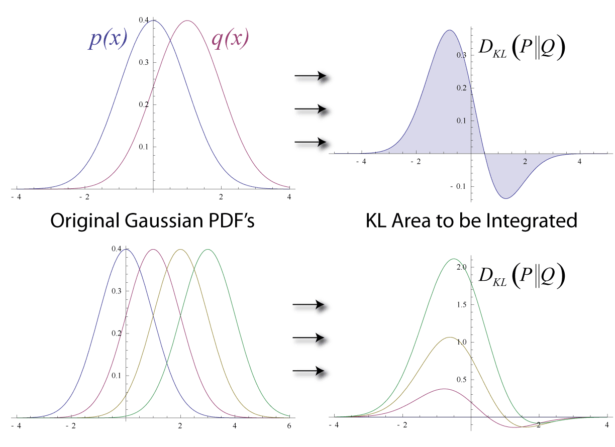
Figure: Distance between two distributions. (Wikipedia)

Given two discrete probability distributions ${\it P}(A)$ and ${\it Q}(B)$ with discrete random variates, $A$ and $B$, having realisations $A=a_{j}$ and $B=b_{j}$, over $n$ singletons $j=1,...,n$. KL divergence or distance $D_{KL}$ in between $P$ and $Q$ is defined as follows:

$D_{KL} = D_{KL}\big({\it P}(A) || {\it Q}(B)\big)=\sum_{j=1}^{n} {\it P}(A=a_{j}) \log \Big( \cfrac{{\it P}(A=a_{j})}{{\it Q}(B=b_{j})} \Big)$

$\log$ is in base $e$.

${\bf Definition}$: Mutual Information on Discrete Random Variates

Two discrete random variables $X$ and $Y$, having realisations $X=x_{k}$ and $Y=y_{l}$, over $m$ and $n$ singletons $k=1,...,n$ and $l=1,...,m$ respectively, are given. Mutual information, $I(X;Y)$ is defined as follows,

$I(X;Y) = \sum_{k=1}^{n} \sum_{l=1}^{m} {\it R}(X=x_{k}, Y=y_{l}) \log \Big(\cfrac{ {\it R}(X=x_{k}, Y=y_{l}) }{ {\it R}(X=x_{k}) {\it R}(Y=y_{l})} \Big)$

$\log$ is in base $e$ and $R$ denotes probabilities.

${\bf Definition}$: Mutual Information on Discrete Random Variates with KL distance

Two discrete random variables $X$ and $Y$. Mutual information, $I(X;Y)$ is defined as follows,

$I(X;Y) = D_{KL} \Big( {\it R}(X, Y) || {\it R}(X) {\it R}(Y) \Big)$

${\bf Problem: Example}$: Given two discrete random variables $X$ and $Y$ defined on the following sample spaces $(a,b,c)$ and $(d,e)$ respectively. Write down the expression for the mutual information, I(X;Y), expanding summation.

${\bf Solution: Example}$:

$I(X;Y) = {\it R}(X=a, Y=d) \log \Big(\cfrac{ {\it R}(X=a, Y=d) }{ {\it R}(X=a) {\it R}(Y=d)} \Big) +$

${\it R}(X=b, Y=d) \log \Big(\cfrac{ {\it R}(X=b, Y=d) }{ {\it R}(X=b) {\it R}(Y=d)} \Big)+$

${\it R}(X=c, Y=d) \log \Big(\cfrac{ {\it R}(X=c, Y=d) }{ {\it R}(X=c) {\it R}(Y=d)} \Big)+$

${\it R}(X=a, Y=e) \log \Big(\cfrac{ {\it R}(X=a, Y=e) }{ {\it R}(X=a) {\it R}(Y=e)} \Big)+$

${\it R}(X=b, Y=e) \log \Big(\cfrac{ {\it R}(X=b, Y=e) }{ {\it R}(X=b) {\it R}(Y=e)} \Big)+$

${\it R}(X=c, Y=e) \log \Big(\cfrac{ {\it R}(X=c, Y=e) }{ {\it R}(X=c) {\it R}(Y=e)} \Big)$

${\bf Definition}$: Two discrete random variables $X$ and $Y$, having realisations $X=x_{k}$ and $Y=y_{l}$, over $m$ and $n$ singletons $k=1,...,n$ and $l=1,...,m$ respectively, are given. Two-way contingency table of realisations of $X$ and $Y$ along the same measured data points, $N$ observations, can be constructed by counting co-occurances, or cross-classifying factors. Normalizing the resulting frequency table will produce joint and marginal probabilities.

                Y=y_{1}              ...    Y=y_{l}              R(X)

    X=x_{1}    R(X=x_{1}, Y=y_{1})   ... R(X=x_{1}, Y=y_{l}) R(X=x_{1})
    X=x_{2}    R(X=x_{2}, Y=y_{1})   ... R(X=x_{2}, Y=y_{l}) R(X=x_{2})
    ...             ...              ...        ...              ...
    X=x_{k}    R(X=x_{k}, Y=y_{1})   ... R(X=x_{k}, Y=y_{1} R(X=x_{k})

    R(Y)        R(Y=y{1})           ... R(Y=y_{l})

Simulated example with R

set.seed(3951824)
# Table of counts (contingency)
X <- sample(letters[1:3], 100, 1)
Y <- sample(letters[4:5], 100, 1)
t  <- table(X,Y)
tp  <- t/100 # proportions
tn  <- tp/sum(tp)     # normalized, joints
p_x <- rowSums(tn)    # marginals
p_y <- colSums(tn)

P <- tn 
Q <- p_x %o% p_y 

# P(X, Y)   : bin frequency: P_i
# P(X) P(Y) : bin frequency, Q_i 
mi <- sum(P*log(P/Q))
library(entropy)
mi.empirical(t) == mi

References

(KullbackLeibler57) Kullback, S.; Leibler, R.A. (1951). "On information and sufficiency". Annals of Mathematical Statistics 22 (1): 79–86.

Monday, 25 July 2016

Economy and dynamic modelling: Haavelmo's approach

Updated on 25 August 2017
Preamable: Predictions using dynamic modelling
Machine Learning and Neural Networks are not the only way to do data science or AI. There are other techniques to explore , for example, from quantitative economics. Apart from Game Theory, dynamic modelling could be suitable to many prediction problems, specially the ones with temporal datasets. Here is one example technique from forgotten Norwegian Nobel prize winning economist/data scientist Trygve Haavelmo. Advantage of such models are they can be explained, not fully black box. Make no mistake, for very large system with large datasets, this is not that trivial to implement, GPUs are well suited. In this post we give one hands on exercise.

Summary

Econometrics aims at estimating observables in the economy and their inter-dependencies and testing the estimates against the economic reality. A quantitative approach to express these inter-dependencies appear as simultaneous equations, an i.e. system of linear equations, this is a mathematical structure of economic relationships that were made possible with the pioneering work of Nobel prize winning economist Trygve Haavelmo [1,2]. This approach and its dynamic variants are now used routinely in dynamic modelling of econometric systems. From a computational perspective, R-project provides efficient and very rich computational environment and the large set of extensions for econometrics in general [3].

Dynamic Modelling

The simplest relationship that can be constructed with two arbitrary economic variables, or instruments, $X(t)$ and $Y(t)$ is shown by Haavelmo [1]. For example, these variables could be unemployment rate and Gross Domestic Product (GDP), as in Okun's law. Hence, the simplest bi-variate simultaneous system of equations looks as follows,

$X(t) =a Y(t) + \epsilon_{x}(t)$,

$Y(t) =b X(t) + \epsilon_{y}(t)$,

where $a$ and $b$ are constant coefficients. Where, $\epsilon_{x}$ and $\epsilon_{y}$, appear as non-deterministic disturbances and are not observed in the modelled economic system. Disturbances are usually expressed as random variables drawn from the normal distribution. At this stage, one can follow two approaches in doing economic scenario analysis for forecasting. We can aim at finding coefficients $a$ and $b$ using economic data via dynamic regression. If $a$ and $b$ coefficients are known, we may want to study effect of different disturbances over time.

Dynamic Haavelmo Model

A model of propensity to consume in economic system is shown by Haavelmo [3] based on his analysis of US economic conditions between 1929-1949. His analysis leads to following simultaneous system of equations,

$c(t)= \alpha y(t) + \beta + u(t)$,
$r(t)= \mu (c(t)+x(t)) +\nu + w(t)$,
$y(t)= c(t)+x(t)-r(t)$,

where $\alpha,\beta,\mu,\nu$ are constants and $u(t)$ and $w(t)$ are disturbances. Economic variables have the following meanings,

c(t) : personal consumption expenditures,
y(t) : personal disposable income,
r(t) : gross business savings,
x(t) : gross investment.

However, this model considered to be static while all the relationships are given at the same time point. Zellner-Palm [5] provided a dynamic version of the Haavelmo's model. Here we write down a version of it,

$c(t)= \alpha Dy(t) + \beta + u(t)$,
$r(t)= \mu D(c(t)+x(t)) +\nu + w(t)$,
$y(t)= c(t)+x(t)-r(t)$.

where difference operator means, $Dy(t) = y(t)-y(t-1)$.

Krokozhia Case Study

Data

Krokozhia is a fictional country depicted in Steven Spielberg's movie The Terminal. Let's generate a fictional data for our dynamic Haavelmo model's economic instruments for this country from 1950 to present in R,

set.seed(4242)
# KH: Krokozhia Haavelmo Model
KH.df <- data.frame(Year=seq(1950,2013),
c=sample(300:1500,64,replace=TRUE),
y=sample(1000:5000,64,replace=TRUE),

r=sample(100:500,64,replace=TRUE),
x=sample(100:500,64,replace=TRUE))
# Add lag data for difference
KH.df$y.lag <- c(NA, KH.df$y[1:63])
KH.df$c.lag <- c(NA, KH.df$c[1:63])
KH.df$x.lag <- c(NA, KH.df$x[1:63])

Determining Constants

Multilevel regression is needed in order to fit the data and determine the constants of the dynamic model. One R package called sem developed by John Fox can do such analysis.

library(sem)
# Two-stage least squares
#   Eq1: $c(t)= \alpha Dy(t) + \beta + u(t)$,
#         \beta is the intercept and u(t) is not used
#   Eq2: $r(t)= \mu D(c(t)+x(t)) +\nu + w(t)$,
#         \nu is the intercept and w(t) is not used
KH.eq1 <- tsls(c~I(y-y.lag), ~c+y+r, data=KH.df)
KH.eq2 <- tsls(r~I(c-c.lag+x-x.lag), ~c+y+r, data=KH.df)
coef(KH.eq1) # alpha=875.414 nu=0.015
coef(KH.eq2) # mu=-0.028      nu=300.675

Here tsls performs two-stage least square analysis.

Propagating a disturbance in the economy

We have not used any disturbance in determining the system coefficients, constants, above. However, we can propagate the values of economic observables using the dynamic model if we set a disturbance value at a given time. Imagine if we set disturbance on the year 2001 as $u=200$ and $w=150$. Hence, the dynamic model will read on year 2001, $t=2001$, $u=200$ and $w=150$

     $c = 875.414 (y-2570) + 0.015 + 200$
   $r = -0.028(c+x-1281-479) + 300.675 + 150$,
   $y = c+x-r$,

By solving this under-determined system of equations we can determine the values in the year 2001 and furthermore propagate all dynamics after 2001 similarly. The resulting new series will give us a quantitative idea of the effect of single disturbance in the simulated economy.

Conclusions and outlook

In this post, we have briefly reviewed possible uses of R in simulating dynamic econometric models, in particular simultaneous equation models. A simple demonstration of determining model coefficients of the Haavelmo type toy model with generated synthetic data is provided. One use case of this type of approach in economic scenario analysis and forecasting is to monitor propagation of the econometric instruments over time is also mentioned.

References

[1] The Statistical Implications of a System of Simultaneous Equations,
     Trygve Haavelmo, Econometrica, Vol. 11, No. 1. (Jan., 1943), pp. 1-12
[2] Econometrics Analysis, William H. Greene, Prentice Hall (2011)
[3] Applied Econometrics with R,
     Kleiber, Christian, Zeileis, Achim, Springer (2008), Achim Zeileis
[4] Methods of measuring the marginal propensity to consume,
     T. Haavelmo, Journal of the American Statistical Association,
     1947 - Taylor & Francis.
[5] Time series analysis and simultaneous equation econometric models,
      Zellner, Arnold and Palm, Franz, Journal of Econometrics,
      Vol.2, Num.1, p17-54 (1974)

Saturday, 16 January 2016

S-shaped data: Smoothing with quasibinomial distribution

Figure 1: Synthetic data and fitted curves.

S-shaped distributed data can be found in many applications. Such data can be approximated with logistic distribution function [1]. Cumulative distribution function of logistic distribution function is a logistic function, i.e., logit.

To demonstrate this, in this short example, after generating a synthetic data, we will fit quasibinomial regression model to different observations.

ggplot [2], an implementation of grammar of graphics [3], provides capability to apply regression or customised smoothing onto a raw data during plotting.

Generating Synthetic Data

Let generate set of $n$ observation over time $t$, denoted, $X_{1}, X_{2}, ..., X_{n}$ for $k$ observation $X=(x_{1}, x_{2}, ..., x_{k})$. We will use cumulative function for logistic distribution [4],
$$F(x;\mu,s) = \frac{1}{2} + \frac{1}{2} \tanh((x-\mu)/2s)$$, adding some random noise to make
it realistic.

Let's say there are $k=6$ observations with the following parameter sets, $\mu = \{9,2,3,5,7,5\}$ and $s=\{2,2,4,3,4,2\}$, we will utilise `mapply` [5] in generating a syntetic data frame.

generate_logit_cdf <- function(mu, s, 
                               sigma_y=0.1, 
                               x=seq(-5,20,0.1)) {
  x_ms <- (x-mu)/s
  y    <- 0.5 + 0.5 * tanh(x_ms)  
  y    <- abs(y + rnorm(length(x), 0, sigma_y))
  ix   <- which(y>=1.0)
  if(length(ix)>=1) { 
    y[ix] <- 1.0
  }
  return(y)
}
set.seed(424242)
x      <- seq(-5,20,0.025) # 1001 observation
mu_vec <- c(1,2,3,5,7,8)   # 6 variables
s_vec  <- c(2,2,4,3,4,2)
# Syntetic variables
observations_df<- mapply(generate_logit_cdf, 
                              mu_vec, 
                              s_vec, 
                              MoreArgs = list(x=x))
# Give them names
colnames(observations_df) <- c("Var1", "Var2", "Var3", "Var4", "Var5", "Var6")
head(observations_df)

Smoothing of observations

Using the syntetic data we have generated, `observations_df`,
we can noq use `ggplot` and `quasibinomial` `glm` to visualise
and smooth the variables.

library(ggplot2)
 library(reshape2)
 df_all <- reshape2:::melt(observations_df)
 colnames(df_all) <- c("x", "observation", "y")
 df_all$observation <- as.factor(df_all$observation)
 p1<-ggplot(df_all, aes(x=x, y=y, colour=observation)) + geom_point() + 
        scale_color_brewer(palette = "Reds") +
        theme(
              panel.background = element_blank(), 
              axis.text.x      = element_text(face="bold", color="#000000", size=11),
              axis.text.y      = element_text(face="bold", color="#000000", size=11),
              axis.title.x     = element_text(face="bold", color="#000000", size=11),
              axis.title.y     = element_text(face="bold", color="#000000", size=11)
#              legend.position = "none"
              )
 l1<-ggplot(df_all, aes(x=x, y=y, colour=observation)) +
        geom_point(size=3) + scale_color_brewer(palette = "Reds") + 
        scale_color_brewer(palette = "Reds") + 
        #geom_smooth(method="loess", se = FALSE, size=1.5) +
        geom_smooth(aes(group=observation),method="glm", family=quasibinomial(), formula="y~x",
                       se = FALSE, size=1.5) +
        xlab("x") + 
        ylab("y") +
        #scale_y_continuous(breaks=seq(0.0,1,0.1)) +
        #scale_x_continuous(breaks=seq(0.0,230,20)) +
        #ggtitle("")  + 
        theme(
              panel.background = element_blank(), 
              axis.text.x      = element_text(face="bold", color="#000000", size=11),
              axis.text.y      = element_text(face="bold", color="#000000", size=11),
              axis.title.x     = element_text(face="bold", color="#000000", size=11),
              axis.title.y     = element_text(face="bold", color="#000000", size=11)
              )
 library(gridExtra)
 gridExtra:::grid.arrange(p1,l1)

References
[1] https://en.wikipedia.org/wiki/Logistic_distribution#Applications
[2] http://www.ggplot.org
[3] The Grammar of Graphics, L. Wilkinson, http://www.amzn.com/038724544
[4] http://en.wikipedia.org/wiki/Logistic_distribution#Cumulative_distribution_function.
[5] https://stat.ethz.ch/R-manual/R-devel/library/base/html/mapply.html

Notes:
* Quasibinomial distribution is as a term used in R's GLM implementation context, see here.