Wednesday, 12 November 2025

Understanding high-entropy random number generation for research: Leymosun Package

Preamble

The idea of generating randomness via computers goes back to von Neumann's and his team of colleagues work in Princeton and Los Alamos. Even though, he was sceptical about the idea of generating randomness via computer programs, this practice is now almost a de-facto standard, so the name pseudo-random-number-generator (PRNG). Is there a way to generate better PRNGs? This is a continuous research. A practical matter of seeding is often ignored because a good PRNG should be reliable regardless of seeding, however, in repeated calls to a random sequence may degrade this view. 

PRNGs bird's eye view : Simulating Randomness

Wigner's Cat (Leymosun Package)
Probably the easiest way to explain RNGs appears to be using discrete recurrence equations, well, actually most RNGs generates numbers based on this, such as $$x_{n+1} = f(x_{n})$$ for example it can be parametrised by $a$ and $b$, $f(x_{n}) = a x_{n} + b$. This basic form allow us remarkably to generate quite useful simulation of randomness. 

Concept of a seed 

An other concept is a seed, it can be the first number to start recurrence but it can also be some other form of something related to random generation, if $x_{0}$ is fixed or has some complicated formula. We usually put seed like 42 or 4242 or some other integer.  There are actually used code with seeds 12345.

Anytime we call a randomisation functions, such as sampling 

How eliminating seeding improves things? High-Entropy Randomness

We use new seeds at each new call, this would generate a different sequence and yields us to sample it. This practice would improve the non-predictability as we sample different sequences. But then the question is, where to get the seeds at each call? The answer lies on the "entropy pool" provided by the operating systems, such us Unix's "/dev/random". Essentially they are kind of random devices we tap into. By using hybrid approach of pseudorandom generation via algorithms and seeding from random devices yields to an increased, High-Entropy randomness. 

Leymosun: Tested implementation

Leymosun Python package provides this facility, using its random module functionality operates as described above and one doesn't need to provide any seeding, it uses non-deterministic seeding. Using NIST's test, we have shown that high-entropy approach gives higher pass scores in randomness tests compare to baseline seeding, such as 42. To install, just use:

 pip install leymosun

Conclusion

Using high-quality randomness for research is quite critical. We have shortly discussed this covering the new approach of using RNGs. 

Further reading and links


Please cite as follows:

@article{suzen21,
  title={Empirical deviations of semicircle law in mixed-matrix ensembles},
  author={S{\"u}zen, Mehmet},
  year={2021},
  journal={HAL-Science},
  url={https://hal.science/hal-03464130/}
}
 @misc{suezen25ley, 
     title = {Understanding high-entropy random number generation for research: Leymosun Package}, 
     howpublished = {\url{https://memosisland.blogspot.com/2025/11/leymosun-high-entropy-randomness.html}}, 
     author = {Mehmet Süzen},
     year = {2025}
}  

Tuesday, 22 April 2025

Numerical stability showcase: Ranking with SoftMax or Boltzmann factor

Preamble 

Image: Babylonian table for
computation (Wikipedia)
Probably, one of the most important aspects of computational work in quantitative fields, such as physics and data sciences is stability of numerical computations. It implies given inputs, outputs should not wildly deviates to large numbers or it must not distort the results, such as ranking based on scores, one of the most used computation in data science tasks, such as in classification of clustering. In this short post, we provide a stunning example of using SoftMax that creates wrong results if it applied naively. 

SoftMax:  Normalisation with Boltzmann factor

SoftMax is actually something more physics concept than a data science usage. The most common usage in data science is used for ranking.  Given a vector $x_{i}$, then softmax can be computed with the following expression read $$exp(x_{i})/\sum_{i} exp(x_{I}).$$ This originates from statistical physics, i.e., Boltzmann factor. 

Source of Numerical Instability

Using exponential function in the denominator in a sum creates a numerical instability, if one of the number deviates from other numbers significantly in the vector. This makes all other entries zero for the output of softmax.  

Example Instability: Ranking with SoftMax

Let's say we have the following scores 

scores = [1.4, 1.5, 1.6, 170]

for teams A, B, C,  D for some metric, we want to turn this into probabilistic interpretation with SoftMax, this will read, [0., 0., 0., 1.] we see that D comes on top but A,B,C are tied. 

LogSoftMax

We can rectify this instability by using LogSoftMax. reads $$\log exp(x_{I})-log(\sum_{i} exp(x_{i})),$$reads [-168.6000, -168.5000, -168.4000, 0.0000], so that we can induce consecutive ranking without ties, as follows D, A, B, C.

Conclusion

There is a similar practice in statistics for likelihood computations, as Gaussians brings exponential repeatedly. Using Log of the given operations will stabilise the numerical instabilities caused by repeated exponentiation. This shows the importance of numerical pitfalls in data sciences. 

Cite as follows

 @misc{suezen25softmax, 
     title = {Numerical stability showcase: Ranking with SoftMax or Boltzmann factor}, 
     howpublished = {\url{https://memosisland.blogspot.com/2025/04/softmax-numerical-stability.html}}, 
     author = {Mehmet Süzen},
     year = {2025}
}  

Appendix: Python method 

A python method using PyTorch computing softmax example from the main text. 

import torch

List = list
Tensor = torch.tensor

def get_softmax(scores:List, log :bool = False) -> Tensor:
"""
Compute softmax of a list

Defaults to LogSoftMax
"""
scores = torch.tensor(scores)
if log:
scores = torch.log_softmax(scores, dim=0)
else:
scores = torch.softmax(scores, dim=0)
return scores


Saturday, 28 September 2024

Matrix language conjecture for combinatorics:
Combinatorial set generation via nested cartesian products

Rubik's cube (Wikipedia)

Preamble
 

Counting is one of the most important concepts in probability and statistical mechanics as well. Two primary characteristics of choosing $n$ items from $N$ items are (no)-order and (no)-repeat. This leads to four  possible cases that leads to combinations and permutations of different kinds to found the resulting set size. Specially the case for repeated no-ordering would be quite hard to memorise or derive on the spot. There is a catch, we can compute the set sizes in combinatorics but usually there is no explicit explanation how could we get the entire combinatorial set member via a computation.  In this short exposition, we have demonstrated a conjecture  that obtaining resulting combinatorial set members is possible via nested cartesian products of the set of the $N$ items: Concepts from matrices help to identify resulting set members in the given combinatorics case.  

Compact Combinatorics

Combinatorics over choosing $n$ items over $N$ has four cases as mentioned. Here is the formulations of choosing sets over $N$ items of size $n$ with different constraints, resulting set sizes will be: 

  • Ordering matters with replacement : $N^n$
  • Ordering matters without replacement: $\Large \frac{N!}{(N-n)!} $
  • Ordering doesn't matter with replacement: $\Large \frac{(n+N-1)!}{n!(N-1)!}$
  • Ordering doesn't matter without replacement: $\Large \frac{N!}{n!(N-n)!} $
However, it is often we forget the formulations of the each case, even to identify the case given a problem.

Obtaining resulting sets: Combinatorial Matrix

We know the size of the resulting sets if we do the choose over a set given $n$. However, the members of the resulting set is not usually known via a computational procedure in standard texts. However, this is possible via cartesian product of the initial set by itself if $n=2$, i.e., pairwise matrices over $N$ item, a combinatorial matrix.     

Matrix language conjecture for combinatorics: A combinatorial matrix has different portions. An entire matrix (E), diagonals (D), upper diagonal (UD) and lower diagonal (LD).  These portions or combinations of them corresponds to the cases above, somehow obvious after a close look: 

  • Ordering matters with replacement : E
  • Ordering matters without replacement: E-D
  • Ordering doesn't matter with replacement:   UD+D or LD+D   
  • Ordering doesn't matter without replacement: UD or LD
By choosing certain portions of the matrix we full-fill constraints of generating new sets. 

Nested Combinatorial Matrices ($n \ge 3$  cases) 

It is obvious that the above conjecture is valid for $n=2$. In the case of where $n \ge 3$ we would need to do more cartesian products over a combinatorial matrix selectively. The idea is as follows: we generate new cartesian products with $N$ items row-wise with removal of the base row at each level due to portions selected. Here is the sketch of the nested cartesian products: 

  1. We start with the case of $n=2$ and generate the matrix.  Retain the corresponding matrix portion.
  2. Then repeat portion for the next levels till exhaustion that items are size $n$: We do cartesian product of the given row to all items again to generate new combinatorial matrix of each element, except the elements deleted from the row due to portion selection, if deleted.
  3. At the end we obtain multiple matrices of possibly different sizes, then choose the portions again to form the resulting set of combinatorial items. 

Conclusion

We have discussed shortly how to leverage a matrix language in finding the resulting sets in core combinatorics counting operations. This could be used as a pedagogical tool, algorithmic development and bringing new relationships between matrices and combinatorial formulaThis is still a conjecture, but taught provoking one that connects matrix generation to combinatorial structures.  

Cite this as follows: 

 @misc{suezen24mcg, 
     title = { Matrix language conjecture for combinatorics: Combinatorial set generation via nested cartesian products}, 
     howpublished = {\url{https://memosisland.blogspot.com/2024/09/combinatorics-touch-of-linear-algebra.html}}
     author = {Mehmet Süzen},
     year = {2024}
}  


Saturday, 1 June 2024

A new kind of AutoML: On the fallacy of many-shot in-context learning with LLMs and PLMs

Extension of this post, appear as a short article with a conjecture:

Preamble 
A graph path (Wikipedia)

With the common usage of  Pre-trained Large  Language Models (PLMs/LLMs), now it is possible to direct them to make data analysis, generate predictions or code for very specialised tasks without training. The primary approach in doing such automated analysis is using many-shot learning. In this short post, it is pointed out that pushing analysis into meta model doesn't remove the analyst, as there are now some claims doing so. This is a common generalisation fallacy in many AI systems. Humans are actually are still in the loop and certain automation presented as if human's are removed entirely is not a fair representation of the capabilities and advantages brought by these models. 

How to direct PLMs to do new-prediction without training?

This is quite an attractive premise. Using a foundational model, we could update their ability of prediction beyond training data by simply inducing a memory in their input, so called Chain-of-Though (CoT). At this point, we can deploy the model for an automated task with invoking CoT before its first prompt. This is a new kind of AutoML approach, that supervised learning takes a new great-look: pushes training efforts to building chain-of-thought datasets. Building CoTs appears to be a meta modelling tasks and requires domain knowledge to develop.

Did we really remove the data analyst, software developer or the practitioner from the loop? 

Short answer is No. What we did by is a new way of performing a specialised task, i.e., modelling is moved into a meta modelling stage. Meaning a memory induced by CoT is  designed by experienced human and it will be broken if the task or input data deviates a little differently. A usual culprit in play here; a reliability is problematic. Even though this is quite a promising development and potential to be a game changer on how we practice machine learning, error-rates are still quite high, see Agarwal-Singh et. al. (2024).  

Conclusion 

In this short exposition, we argue that many-shot learning, chain-of-thought learning for foundation models is actually a new kind of AutoML tool. AutoML doesn't imply that human expert is removed from the picture completely. However it greatly assist the scientist, analyst, programmer or practitioner, in automating some tasks as meta programming tool. It will also help less-experienced colleague to start being a bit more productive. These tools indeed improves our computational tool boxes, specifically as a new AutoML tool.  

Further reading

Please cite as follows:

 @misc{suezen24pmlauto, 
     title = {A new kind of AutoML: On the fallacy of many-shot in-context learning with LLMs and PLMs}, 
     howpublished = {\url{https://memosisland.blogspot.com/2024/05/llm-analysis-fallacy.html}, 
     author = {Mehmet Süzen},
     year = {2024}
}  

Saturday, 24 February 2024

Inducing time-asymmetry on reversible classical statistical mechanics via Interventional Thermodynamic Ensembles (ITEs).

Preamble 

Probably, one of the most fundamental issue in classical statistical mechanics is extending reversible dynamics to many-particle systems that behaves irreversibly. In other words, how time's arrow appears even though constituted systems evolves in reversible dynamics. This is the main idea of Loschmidt's paradox. The resolution to this paradox lies into something called interventional thermodynamic ensembles (ITEs).  

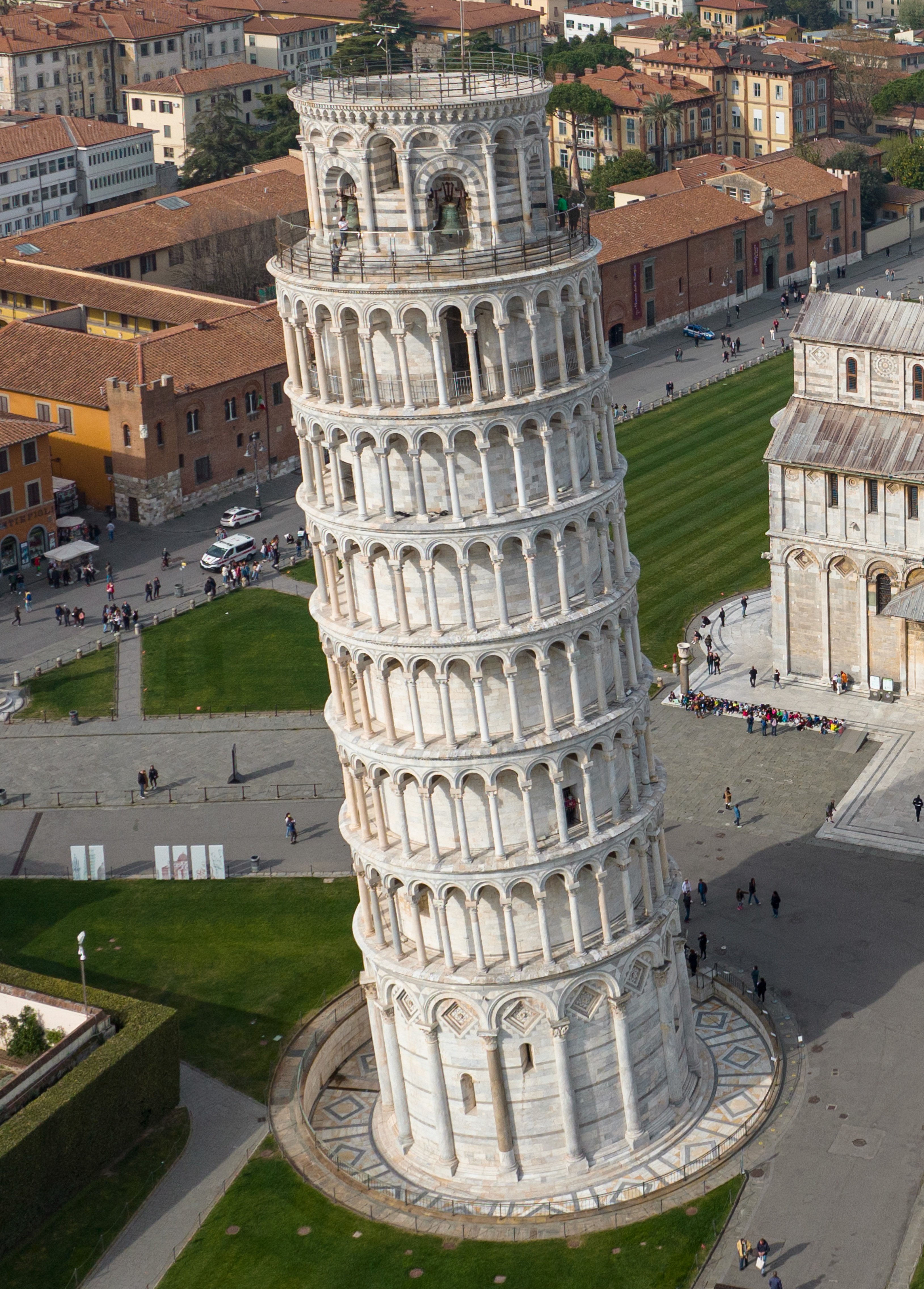
Leaning Tower
of Pisa:Recall Galileo's 
Experiments
 (Wikipedia)

Time-asymmetry is about different histories : Counterfactual dynamics

Before trying to understand how ITEs are used in resolving Loschmidt's paradox, we understand that inducing different trajectories on an identical dynamical system in "a parallel universe" implies time-asymmetry. A trajectory provides here a reversibility.  So called "a parallel universe" is about imagining a different dynamics via a sampling, this corresponds to counterfactuals within Causal inference frameworks. 

Interventional Thermodynamic Ensembles (ITEs)

Interventional ensemble build upon an other ensemble, for the sake of simplicity, we can think of an ensemble as an associated chosen sampling scheme. From this perspective,  sampling scheme $\mathscr{E}$ would have an interventional sampling $do(\mathscr{E})$ if the adjusted scheme only  introduces a change in the scheme that doesn't change the inherent dynamics but effects the dynamical  history. One of the first examples of this is appeared recently: single-spin-flip vs. dual-spin-flip dynamics [suezen23]. This is shown with simulations. 

Outlook

Reversibility and time-asymmetry in classical dynamics are a long standing issues in physics. By inducing causal inference perspective in computing dynamical evolution of many body systems leads to reconciliation of reversibility and time-asymmetry i.e., $do-$operator's interpretation.

References

[suezen23] H-theorem do-conjecture (2023) arXiv:2310.01458 (simulation code GitHub).

Please Cite as:

 @misc{suezen24ite, 
     title = {Inducing time-asymmetry on reversible classical statistical mechanics via  Interventional Thermodynamic Ensembles (ITEs)}, 
     howpublished = {\url{https://memosisland.blogspot.com/2024/02/inducing-time-asymmetry-on-reversible.html}, 
     author = {Mehmet Süzen},
     year = {2024}
}  


Friday, 9 February 2024

Exact reproducibility of stochastic simulations for parallel and serial algorithms simultaneously
Random Stream Chunking

Preamble 

Figure: Visual description of
random stream chunking, M.Suzen (2017)
The advent of using computational sciences approaches, i.e., data science and machine learning, in the industry becomes more common practice in almost all organisations due to the democratisation of data science tools and availability of inexpensive cloud infrastructure. This brings the requirement or even compulsory practice of a code being so called parallelised. Note that parallelisation is used as an umbrella term here for using multiple compute resources in accelerating otherwise a serial computation and could mean a distributed or multi-core computing, i.e., multiple CPUs/GPUs. Here we provide a simple yet a very powerful approach to preserve reproducibility of parallel and serial implementation of the same algorithm that uses random numbers, i.e., stochastic simulations. We assume Single Instruction Multiple Data (SIMD) setting. 

Terminology on repeatability, reproducibility and  replicability 

Even though we only use reproducibility as a term as an umbrella term, there are clear distinctions, recommended by ACM, here. We summarise this from computational science perspective :

repeatability : Owner re-run the code to produce the same results on own environment. 
reproducibility: Others can  re-run the code to produce the same results on other's environment. 
replicability: Others can re-code the same thing differently and produce the same results on other's environment. 

In the context of this post, since parallel and serial settings would constitute different environments, the practice of getting the same results, this falls under reproducibility.   

Single Instruction Multiple Data (SIMD) setting. 

This is the most used, and probably the only one you would ever need, approach in parallel processing. It implies using the same instruction, i.e., algorithm or function/module, for the distinct portions of the data. This originates from applied mathematics techniques so called domain decomposition method

Simultaneous Random Stream Chunking 

The approach in ensuring exact reproducibility of a stochastic algorithm in both serial and parallel implementation lies in default chunking in producing the random numbers both in serial and parallel code. This approach used in the Bristol Python package Here is the mathematical definition. 

Defintion Random Stream Chunking Given a random number generator $\mathscr{R}(s_{k})$ with as seed $s_{k}$ is used over $k$-partitions. These partitions are always corresponds to $k$ datasets, MD portion of SIMD. In the case of parallel algorithms, each $k$ corresponds to a different compute resource     $\mathscr{C}_{k}$. 

By this definition we ensure that both parallel and serial processing receiving exactly the same random number, this is summarised in the Figure.

Conclusion

We outline a simple yet effective way of ensuring exact reproducibility of serial and parallel simulations simultaneously. However, reproducibility of stochastic simulations are highly hardware dependent as well, such as GPUs and NPUs, and their internal streams might not be that easy to control partitions, but generic idea presented here should be applicable.


Please cite this article as: 

 @misc{suezen24rep, 
     title = {Exact reproducibility of stochastic simulations for parallel and serial algorithms simultaneously}, 
     howpublished = {\url{https://memosisland.blogspot.com/2024/02/exact-reproducibility-of-stochastic.html}, 
     author = {Mehmet Süzen},
     year = {2024}
}


Tuesday, 28 November 2023

What's the purpose of randomness in causal discovery techniques?

Roulette
Wheel (Wikipedia)

Preamble
 

In this short exposition, we inquire about the purpose of randomness and how this related to discovering or testing causal inferential problem solving using data and causal models. In his seminal work by Holland (1986) point out something striking that was not put in such form earlier works. He stated the "obvious" that almost all data sets addressing interventional nature, such as treatment vs. non-treatment, that a person or unit we study, can not be treated and not-treated at the same time. We delve question of randomness from this perspective, i.e., so called fundamental problem of causal inference.

Group assignment for causal inference   

Group assignment probably one of the most fundamental approach in statistical research, such as in the famous Lady tea tasting problem.  The idea of assignment in causal inference, we need to find a matching person or unit that is not-treated if we have a treated sample or the other-way around, so called a matching or balancing.  

Randomness in causality: Removal of  pseudo-confounders

Randomness doesn't only allow fair representation of control and treatment group assignments, reducing bias essentially. The primary effect of randomness is removal of  pseudo-confounders, this is not well studied in the literature. What it means, if we don't randomise there would be other causal connections that would really shouldn't be there. 

Conclusion

Here, we hint about something called  pseudo-confounders.  Randomisation in both matching and other causal techniques primarily removes bias but  removal of pseudo-confounders is not commonly mentioned and an open research.

Further reading

Please cite this article as: 

 @misc{suezen23ran, 
     title = {What's the purpose of randomness in causal discovery techniques?}, 
     howpublished = {\url{https://memosisland.blogspot.com/2023/11/causal-inference-randomisation.html}, 
     author = {Mehmet Süzen},
     year = {2023}
}


Saturday, 25 November 2023

Why should there be no simultaneity rule for causal models?

Dominos in motion
(Wikipedia)

Preamble
 

The definition of weighted directed graphs (wDAGs) provides a great opportunity to express causal relationships among given variates. Usually this is expressed as SCMs, Structural Causal Model or in more generally causal model. A given causal model can be expressed as set of simultaneous equations, given a direction for the equality, right to left , meaning $A=B$ implies B causes A to happen  $B \to A$ . Then what happens if A is a function of B and C, $A=f(B,C)$, then we say $ B \to A$ and $C \to A$ occurs simultaneously.  In this post we discuss this situation that there should be no simultaneity rule in causal models, regardless of if they are not time-series models.

Understanding  causal models

Basic definition of a causal model follows a functional form with set of equations, realistically with added noise. The models forms a weighted Directed Acyclic Graphs (wDAGs) visually. Here is the mathematical definition due to Pearl (Causality 2009), we made it a bit more coarser in this definition: 

Definition (Causal Model) : Given set of $n$-variables $X \in \mathbb{R}^{n}$, two subsets of $X= x_{1} \cup x_{2}$, they can form set of equations $x_{2}=f(x_{1}; \alpha; \epsilon)$,  $\alpha$ being the causal effect sizes on $x_{1}$ as causes of $x_{2}$ with some noise $\epsilon$. This corresponds to a $wDAG$ formed among $X$ with weights $\alpha$. So that there is a graph $\mathscr{G}(X, \alpha)$ representing this set of equations, where by equality put direction from right to the left side of the equation. 

However this definition does not set any constraints on the values of $\alpha$. Any two or more values of $\alpha$-s can be equivalent on the same path within $X$. This implies an interestingly that there would be set of variates simultaneously causes the same thing. It sounds plausible and physically possible to a degree within Planck-time. However, this brings an ambiguity of breaking ties in ordering events.

Perfect Causal Ordering

Given wDAG as a causal model induces causal ordering among all members of $X$. As we defined how this can be achieved in a recent post: Practical causal ordering. In this context, perfect causal ordering implies  $\alpha$ values within the first order paths to a given end variable are different. Mathematically speaking a definition follows. 

Definition (No simultaneity rule) Given all $k$ triplets ($x_{i}, y, \alpha_{i}$), that $x_{i}$ is one of the causes of $y$, and $\alpha_{i}$ causal effect sizes, all $\alpha_{i}$ are different numbers, inducing a perfect causal ordering.

This rule ensures we don't need to break ties randomly as causal ordering is established uniformly.

Conclusion: Importance of no simultaneity 

By this definition we ruled out any simultaneous causes. This may sound too restrictive for modelling but this impacts decision making significantly; ranking causes of an outcome will impact how to prioritise the policy in addressing the outcome, i.e., such as medical intervention to prevent first cause. Also, it may not be feasible to intervene simultaneous causes. Hence, establishing primary causes in order is paramount in decision making and execution of any reliable policy.


Further reading

Please cite this article as: 

 @misc{suezen23nos, 
     title = {Why should there be no simultaneity rule for causal models?}, 
     howpublished = {\url{https://memosisland.blogspot.com/2023/11/causal-model-simultaneous.html}, 
     author = {Mehmet Süzen},
     year = {2023}
}


Saturday, 14 October 2023

Ising-Conway lattice-games: Understanding increasing entropy

Preamble

The entropy is probably one of the most difficult physical concepts to grasp. Its inception roots in efficiency of engines and foundational connection to multi-particle classical mechanics to thermodynamics,  i.e., kinetic theory to thermo-statistics. However, computing entropy for a physical systems is a difficult task, as most of the real-physical systems lacks the explicit formulation. Apart from advanced simulation techniques that invokes thermodynamical expressions, pedagogically accessible and physically plausible system is lacking in the literature. Addressing this, we explore here, recently proposed Ising-Conway Games.

Figure: Evolution of Ising-Conway
Game  (arXiv:2310.01458)
Ising-Conway Lattice-Games (ICG)

Ising-Lenz model is probably one of the landmark models in physics, remarkably provides beyond its idealised case of magnetic domains,  now impacts even quantum computational research. However, computing entropy of Ising-Lenz models are still quite difficult. On the other hand, Conway introduce a game with simple rules generating complexity in various orders, via simple dynamical rules. By analogy to these two modelling approach,  we recently introduce game like physical system of spins or lattice sides on a finite space with constraints. This gives a physically plausible dynamics but simpler dynamical evolution to generate the trajectories. Because vanilla Ising-Models requires more complicated Monte Carlo techniques.  Here is the configuration and dynamics of Ising-Conway games,

  1. $M$ sites as a fixed space.
  2. $N$ occupied sites, or 1s.  
  3. Configuration $C(M,N,t)=C(i)$ over time changes. But at $t=0$ all occupied sites live in at the corner.
  4. Configuration can only change to neighbouring sites if they are empty. This is closely related to spin-flip dynamics of the Ising Model. 
  5. No sites occupy the same lattice cell, Pauli exclusion
  6. Should be contained within $M$ Cell.
An example evolution is shown on the Figure.

Defining ensemble Entropy on ICG

Now we are in position to define the entropy for ICGs, which easy to grasp conceptually and computationally.  $C(i, t) \in \{1,0\}$ defines the states of  the game. We build an ensemble at a given time $t$ by defining a region enclosed by 1s.  Then dimensionality of the ensemble  $ k(t) = argmax[\mathbb{I}(C(i))] - argmin [\mathbb{I}(C(i)) ]$. Here,  $\mathbb{I}$ returns index of $1$s on the lattice. This ensemble closely track maximum entropy of the system at a given time. 

Conclusions

A new game-like system that helps us to understand entropy increase that has a plausible physical characteristics that one can easily simulate.

Further reading

  • H-theorem do-conjecture, M.Süzen, arXiv:2310.01458
  • Effective ergodicity in single-spin-flip dynamics, Mehmet Süzen. Phys. Rev. E 90, 03214 url
  • do_ensemble module provides such simulation via simulate_single_spin_flip_game  from the repo h-do-conjecture 

Please cite as 

 @misc{suezen23iclg, 
     title = {Ising-Conway lattice-games: Understanding increasing entropy}, 
     howpublished = {\url{https://memosisland.blogspot.com/2023/10/ising-conway-games-entropy-increase.html}}, 
     author = {Mehmet Süzen},
     year = {2023}
}  


Saturday, 9 September 2023

Practical causal ordering:
Why weighted-Directed Acyclic Graphs (DAGs) are powerful for causal inference?

Preamble 

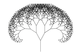
Fractal Tree (Wikipedia)
A quiet causal inference revolution is underway in industry. We see immense success of transformers deep learning architectures. However their success should also be attributed to causal modelling. Large Language Models (LLMs), specially closed-sourced ones, elevates their performance with encoding causal mechanism with human designed deep learning components, i.e., innovative layers such as causal convolutions with multi-head self-attention layers. Now a classical approach,  one of the corner-stone of causality, is expressing modelling variates' causal relationships with  Directed Acyclic Graphs (DAGs). This lead to causal analysis and preserving ordering. In this short tutorial, we cover these without graph theoretic language for practical causal ordering.

Understanding weighted Directed Acyclic Graphs (wDAGs) as causal data structure  

We first define what is a directions and weights. Providing a notational definition via tuples of objects.    

Definition (wDAG): A weighted Directed Acyclic Graph (wDAG)  $\mathscr{G_{c}}$  is defined as set of ordered triplets of weights and connected random variables, such that, $k$th  triplet $(w_{k}, x_{i}, x_{j})$ where by $w_{k} \in \mathbb{R}$ is the weight, an effect size, between two variates that $x_{i}$ effects $x_{j}$. There are constraints : 

(i) No cyclic effects can be defined, necessarily $x_{i}$ can not be equal to $ x_{j}$.

(ii) If there is a definition,  $(w_{k}, x_{i}, x_{j})$ the reverse can't be defined, i.e.,  so that $(w_{k}, x_{j}, x_{i})$ does not exist.    

(iii) No two causal effects sizes can't be exactly equal, $w_{k}$ can not be equal to $w_{l}$, from the same causal variable,  meaning no simultaneous events caused by the same random variable. This prevents ambiguity of ordering and random tie-breaks are unnatural.

This definition is practical and do not introduce any graph theory jargon. We left the sizes of indices as an exercise. 

Inducing Causal Order via wDAGs

By the very definition of wDAGs, the power of this definition is one can construct causal ordering. 

Definition (Causal Ordering from wDAG): Given $\mathscr{G_{c}}$, we can construct causal ordering among random variates $O(i)$ for $x_{i}$ using directionality and weights from  $\mathscr{G_{c}}$:

(i) if there exist a triplet  $(w_{k}, x_{i}, x_{j})$, then ordering $x_{j} \succ x_{i}$, implies $x_{j}$ occurred before $x_{j}$, or cause of $x_{i}$ was $x_{j}$

(ii) if there are two or more triplets having the same first variates, ordering is induces by the effect size $w_{k}$ among them.


To provide a simple example, let's say we formed  a wDAG, $\mathscr{G_{c}} = \{ (0.1, x_{1}, x_{2}),(0.2, x_{1}, x_{3}), (1.1, x_{2}, x_{4})  \}$ then the following causal ordering is established  $x_{1} \succ x_{3} \succ x_{2} \succ x_{4}$, note the ordering of $x_{3}$ that took precedence on $x_{2}$ due to its weight.

Why LLMs with causal ordering are so successful?

Probably not very well spelled property of LLMs are having causal layers with deep learning elevating their ability to capture causal ordering in natural language so well, not only sequence. This is still in infancy from research perspective as LLMs are biologically not plausible engineered software systems act as lossy knowledge compressors, lossy part usually identified as hallucination. 

Conclusion

We introduce basic definition of wDAGs without heavy graph theory jargon and provide hints on why causal ordering with wDAGs has an immense contribution in constructing useful LLMs.

Further reading

  • looper : Causality Resource List. [link]
  • Pearl et. al. Causal Inference in Statistics [link]
  • Shimizu et. al., A Linear Non-Gaussian Acyclic Model for Causal Discovery [link]
  • Hamad, et. al, Dilated causal convolution with multi-head self attention for sensor human activity recognition [link].
  • Lui et. al DecBERT: Enhancing the Language Understanding of BERT with Causal Attention Masks [link]
Please cite as follows:

 @misc{suezen23pco, 
     title = {Practical causal ordering: Why weighted-Directed Acyclic Graphs (DAGs) are powerful for causal inference? }, 
     howpublished = {\url{https://memosisland.blogspot.com/2023/09/causal-ordering-dags-.html}}, 
     author = {Mehmet Süzen},
     year = {2023}
}  

Postscript Notes
Last Update 30 Oct 2024
  • Transformers mathematically mimics wDAGs, i.e., induce causal ordering among distributed representations via “Attention” i.e., weighting inputs and linking them to different types of output sequences.  
  • Directed Acyclic Graphs (DAGs), are actually build implicitly by transformer architectures. This lead to causal analysis and preserving ordering of most meaningful word embeddings in an empirical level, i.e., heuristic causality bound by data-driven model with inductive bias of the modeller (LLM trainer). Striking enough, it is possible to express these relationships using triplet notation without Graph Theory, and that’s what attention layer store rather than graph.
  • The primary  driver in this is not that it can only place an attention to certain portions of the embedded vector space for approximating  the separation of meaning. These data processing instructions actually builds a causal mappings among sub-spaces, i.e., a causal ordering among embedding sub-spaces. In short, transformers are heuristically executing causal discovery.  
  • Transformers in the context of machine translations performs 'causal graph discovery' heuristically, inducing causal ordering. That's why they exceeded previous translation architectures.
    • Grateful to see Judea Pearl's kind note on this via twitter. "What's the input? Statistical data or human authored texts? What are the assumptions behind the discovery?
      • This is critical as not to jump in conclusion that these neural network layers can do causal discovery automatically, but rather in human supervised conditions. The answer was, "Assumption is using an established causal model -human text/translation, directionality is already established. Then transformer compute weights on this graph. Other enabler is word embeddings & large examples. Can't do causal inference as in SCMs, still a statistical model."
      •  Self-attention for LLMs acts as casual discovery machines over human experience

        The success of transformers deep learning architecture can also be attributed to causal modelling. But how?  Probably the most prominent  application of transformers in machine translation. As translation models trained on human translated data

        Causality is inbuilt in these datasets and transformers behave as causal discovery layers. We could imagine weights on the translation matrix and other query matrices as DAGs, as connection between connectivity matrices and graphs are well known. Directionality is dictated by asymmetric weights. This manifest as causal analysis  preserving ordering of most meaningful words embeddings empirically i.e., heuristic causality. This can be demonstrated by triplets without graph theoretic notation, that would induce as causal ordering discovery.

        Causal set theory is also quite striking in quantum gravity. DAGs appear as Partially-ordered sets of events in Planck-scale relativistic events within the discrete space-time. Monograph by Benjamin Dribus, Discrete Causal Theory, Springer (2017)


Tuesday, 22 June 2021

Full cross-validation and generating learning curves for time-series models

Kindly reposted to KDnuggets by Gregory Piatetsky-Shapiro

Preamble

Time-series analysis is needed almost in any quantitative field and real-life systems that collects data over time, i.e., temporal datasets. Building predictive models on temporal datasets for future evolution of systems in consideration are usually called forecasting. The validation of such models deviates from the standard holdout method of having random disjoint splits of train, test and validation sets used in supervised learning. This stems from the fact that time-series are ordered and order induces all sorts of statistical properties that should be retained. For this reason, applying direct cross-validation to time-series model building is not possible and only restricted to out-of-sample (OOS) validation, using the end-tail of a temporal set as a single test set. A recent work proposed an approach that overcomes the known limitation achieving full cross-validation for time-series. The approach opens up for a possibility to produce learning curves for the time-series models as well, which is usually also not possible due to similar reasons.

Reconstructive Cross-validation (rCV) : A meta-algorithm design principles

rCV is proposed recently in the paper titled Generalised learning of time-series: Ornstein-Uhlenbeck processes. The design principles of rCV for time-series aims at the following principles:

   Figure 1 : rCV meta-algorithm for time-series
cross-validation and learning curves.

  1. Logically close to standard cross-validation: Arbitrary test-set size and number of folds. 
  2. Preserve correlations and data order. 
  3. Does not create absurdity of predicting past from the future data. 
  4. Applicable in generic fashion regardless of learning algorithm. 
  5. Applicable to multi-dimensional time-series. 
  6. Evaluation metric agnostic.

Idea of introducing missing-data  : Temporal cross-validation and learning curves

The key idea of rCV is to create cross-validation sets via creating missing-data sets K-times, as in K-fold, with a given degree of missing ratio, i.e., random data point removal. Each fold will have disjoint set of missing data points. By an imputation method, we would fill out the K-disjoint missing data sets and generate K-different training datasets.  This would allow us to have K-different models and we could measure the generalised performance of the modelling approach by testing the primary models prediction on the Out-of-sample (OOS) test set. To avoid confusion about what is a model?, what we are trying to achieve is to find out hypothesis, i.e., the modelling approach.  By changing the ratio of missing data and repeating the cross-validation exercise will yield to set of ratio of missing-missing data introduced and their corresponding rCV errors, the plot is nothing but a learning-curve from supervised learning perspective.  Note that the imputation and prediction models are different models. The primary model we are trying to build is the prediction model we used for producing OOS predictions. The procedure is summarised in Figure 1. 


    Figure 2 : Synthetic data and reconstructions. 


Show-case with Gaussian process models on Ornstein-Uhlenbeck processes


To demonstrate the utility of rCV, the mentioned paper uses a synthetic data generated by Ornstein-Uhlenbeck process, i.e., Gaussian process with certain parameter setting.  Figure 2, shows the synthetic data and example locations of generated missing-data sets's reconstruction errors. Figure 3 shows learning curves depending on the different ratios of missing data setting. 

    Figure 3: Learning curves for the Gaussian Process model
generated by rCV.


Conclusion

rCV provides logically consistent way of practicing cross-validation in time-series. It is usually not possible to produce learning-curves on the same time-window for time-series model: by using rCV with different ratio missing data achieves this as well. rCV paves way to do generalised learning for time-series.

Further Reading

Apart from the paper Generalised learning of time-series: Ornstein-Uhlenbeck processes. the results can be reproduced with the Python prototype implementation,  here.

Tuesday, 29 December 2020

Practice causal inference: Conventional supervised learning can't do inference

Domino OR-gate (Wikipedia)
Preamble

A trained model may provide predictions about input values it may never seen before but it isn't an inference, at least for 'classical' supervised learning. In reality it provides an interpolation from the training-set, i.e., via function approximation: 

Interpolation doesn't mean to have all predictions within  convex-hull of the training set but interpolation as in numerical procedure of using training data only.

What does inference means? 

By inference, "we imply going beyond training data", reference to distributional shift, compositional learning or similar type of learning, should have been raised. This is specially apparent, for example, a human infant may learn  how 3 is similar to 8, but without labels supervised learning in naïve setting can't establish this, i.e., MNIST set without 8 can not learn what is 8 in plain form.

In the case of ontology inference, ontology being a causal graph, that is a "real" inference as it symbolically traverse a graph of causal connections. 

Outlook

We might be able to directly transfer that to regression scenario but probably it is possible with altering our models with SCMs and hybrid symbolic-regression approach. 

Postscript
  • Looper repo provides a resource list for causal inference looper 
  • Thanks to Patrick McCrae for invoking ontology inference comparison.
Cite

 @misc{suezen20pci, 
     title = {Practice causal inference: Conventional supervised learning can't do inference}, 
     howpublished = {\url{https://memosisland.blogspot.com/2020/12/practice-causal-inference-conventional.html}, 
     author = {Mehmet Süzen},
     year = {2020}
}
  

Sunday, 1 November 2020

Gems of data science: 1, 2, infinity

 Summary

Figure: George Gamow's book. (Wikipedia)
Problem-solving is the core activity of data science using scientific principles and evidence. On our side, there is an irresistible urge to solve the most generic form of the problem. We do this almost always from programming to formulation of the problem. But, don't try to solve a generalised version of the problem. Solve it for N=1 if N is 1 in your setting, not for any integer: Save time and resources and try to embed this culture to your teams and management. Extent later when needed on demand.

Solving for N=1 is sufficient if it is the setting


This generalisation phenomenon manifests itself as an algorithmic design: From programming to problem formulation, strategy and policy setting. The core idea can be expressed as mapping, let's say the solution to a problem  is a function, mapping from one domain to a range 

$$ f : \mathbb{R} \to \mathbb{R} $$

Trying to solve for the most generic setting of the problem, namely multivariate setting

$$ f : \mathbb{R}^{m} \to \mathbb{R}^{n} $$

where $m, n$ are the integers generalising the problem.  

Conclusion

It is elegant to solve a generic version of a problem. But is it really needed? Does it reflect reality and would be used? If N=1 is sufficient, then try to implement that solution first before generalising the problem. An exception to this basic pattern would be if you don't have a solution at N=1 but once you move larger N that there is a solution: you might think this is absurd, but SVM works exactly in this setting by solving classification problem for disconnected regions.

Postscripts

  • The title intentionally omits three, while it is a reference to Physics's inability to solve, or rather a mathematical issue of the three-body problem.


Sunday, 28 June 2020

Conjugacy and Equivalence for Deep Neural Networks: Architecture compression to selection

Preamble


A recently shown phenomenon can classify deep learning architectures with only using the knowledge gained by trained weights [suezen20a]. The classification produces a measure of equivalence between two trained neural network and astonishingly captures a family of closely related architectures as equivalent within a given accuracy. In this post, we will look into this from a conceptual perspective. 


Figure 1: VGG architecture spectral difference in the long
positive tail [suezen20a]
The concept of conjugate matrix ensembles and equivalence


Conjugacy is a mathematical construct reflecting different approaches to the same system should yield to the same outcome: It is reflected in the statistical mechanic's concept of ensembles. However, for matrix ensembles, like the ones offered in Random Matrix Theory, the conjugacy is not well defined in the literature. One possible resolution is to look at the cumulative spectral difference between two ensembles in the long positive tail part of the spectrum [suezen20a]. If this is vanishing we can say that two matrix ensembles are conjugate to each other. We observe this with matrix ensembles VGG vs. circular ensembles. 


 Conjugacy is the first step in building equivalence among different architectures.  If two architectures are conjugate to the same third matrix ensemble and their fluctuations on the spectral difference are very close over the spectral locations, they are equivalant in a given accuracy [suezen20a].


Outlook: Where to use equivalence in practice?

The equivalence can be used in selecting or compressing an architecture or classify different neural network architectures. Python notebook to demonstrate this with different vision architecture in PyTorch is provided, here.

Reference


[suezen20a] Equivalence in Deep Neural Networks via Conjugate Matrix Ensembles, Mehmet Suezen, arXiv:2006.13687 (2020)


(c) Copyright 2008-2024 Mehmet Suzen (suzen at acm dot org)

Creative Commons License
This work is licensed under a Creative Commons Attribution 4.0 International License